Polynomial Regression in R Programming (original) (raw)

Last Updated : 15 Jul, 2025

Polynomial Regression is an extension of linear regression where the relationship between the dependent variable (y) and the independent variable (x) is modeled as an nth degree polynomial.

Equation:

y = \beta_0 + \beta_1 x + \beta_2 x^2 + \ldots + \beta_n x^n + \varepsilon

• y: Predicted output (dependent variable)
• \beta_0: Intercept (value of y when x=0)
• \beta_1, \beta_2, \ldots, \beta_n: Coefficients for each power of x
• x, x^2, \ldots, x^n: Input variable and its powers
• \varepsilon: Error term (random noise not captured by the model)

Why Polynomial Regression is Needed

Linear regression assumes a straight-line relationship, but fails to capture underlying trends when the data follows a non-linear pattern.

• **Low prediction accuracy: The model makes poor estimates of the target values.
• **High error rates: The difference between predicted and actual values is large.
• **Underfitting: The model is too simple to capture the underlying pattern in the data.

Implementing Polynomial Regression in R

We can implement Polynomial Regression in R by following a series of steps to prepare the data, build the model and evaluate its performance.

1. Installing Required Packages

We install the tidyverse and caret packages for data manipulation, visualization and machine learning tasks.

• **tidyverse: Used for data wrangling and plotting.
• **caret: Used for simplifying training, tuning and evaluating models. R `

install.packages("tidyverse") install.packages("caret") library(tidyverse) library(caret)

`

2. Loading the Dataset

We load the Boston housing dataset from the MASS package.

• **Boston: Contains housing data for regression modeling. R `

library(MASS) data("Boston")

`

3. Splitting the Data

We split the data into training and test sets using createDataPartition() from the caret package.

• **createDataPartition(): Used to randomly split the data while preserving the distribution. R `

set.seed(123) trainIndex <- createDataPartition(Boston$medv, p = 0.8, list = FALSE) train.data <- Boston[trainIndex, ] test.data <- Boston[-trainIndex, ]

`

4. Building the Polynomial Regression Model

We build a polynomial regression model with degree 2 and 5 using lm().

• **lm(): Fits linear and polynomial regression models.
• **I(): Used to explicitly define powers in formula.
• **poly(): Generates orthogonal polynomials when raw = FALSE, raw powers when TRUE. R `

model2 <- lm(medv ~ lstat + I(lstat^2), data = train.data) model5 <- lm(medv ~ poly(lstat, 5, raw = TRUE), data = train.data)

`

5. Making Predictions

We make predictions on the test data using the predict() function.

• **predict(): Generates predicted values based on the model and new data. R `

pred2 <- predict(model2, test.data) pred5 <- predict(model5, test.data)

`

6. Evaluating Model Performance

We evaluate model accuracy using RMSE and R² with the postResample() function.

• **postResample(): Calculates RMSE and R-squared from predicted and actual values. R `

postResample(pred2, test.data$medv) postResample(pred5, test.data$medv)

`

**Output:

Output

7. Visualizing the Polynomial Fit

We use ggplot2 to plot the data and overlay the polynomial regression curve.

• **stat_smooth(): Adds a smoothed conditional mean (like a regression curve) to the plot. R `

ggplot(train.data, aes(lstat, medv)) + geom_point() + stat_smooth(method = lm, formula = y ~ poly(x, 5, raw = TRUE))

`

**Output:

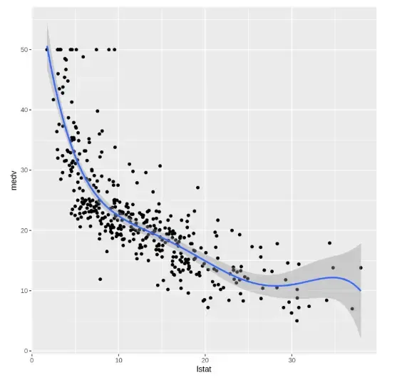
Output

The graph shows a scatterplot of medv vs. lstat with a 5-degree polynomial regression curve overlaid using stat_smooth(). It visually demonstrates how well the model captures the non-linear relationship in the data.

Applications of Polynomial Regression

Polynomial regression is commonly applied in fields where relationships between variables are inherently non-linear, such as:

• **Sales forecasting: Models non-linear trends in revenue or product demand over time.
• **House price prediction: Captures complex relationships between property features and price.
• **Weather modeling: Fits curved patterns in temperature, rainfall, or pollution data.
• **Engineering analysis: Models physical phenomena like stress-strain or motion trajectories.
• **Medical growth tracking: Analyzes non-linear growth patterns in biological data.