Random Forest Approach for Classification in R Programming (original) (raw)

Last Updated : 15 Jul, 2025

Random Forest is a machine learning algorithm used for classification and regression tasks. It creates multiple decision trees and combines their outputs to improve accuracy and minimize overfitting. Each tree makes an individual prediction and the final result is determined by aggregating the predictions from all trees. This method increases the model's reliability, robustness and performance compared to single decision trees. Random Forest is commonly used for its ability to handle large datasets, capture complex relationships and deliver accurate results with minimal tuning.

Key Features of Random Forest

• **Aggregates Multiple Decision Trees: combining predictions to increase model accuracy and stability.
• **Reduces Overfitting: By using multiple trees trained on different data samples, Random Forest reduces overfitting and improves generalization.
• **Handles Missing Data: Random Forest can handle missing values by averaging results from all decision trees.
• **Feature Importance: Random Forest evaluates the importance of each feature, helping identify key predictors for the target variable.

Implementing Random Forest Approach for Classification in R

We will implement the Random Forest approach for classification in R programming. We classify the species of iris plants based on various features using the Random Forest approach in R.

1. Installing and Loading Required Libraries

We will first need to install the randomForest package. We can do this with the following command:

R `

install.packages("randomForest") install.packages("ggplot2")

library(randomForest) library(ggplot2)

`

2. Loading the Dataset

We will use the iris dataset which is a built-in dataset in R and display first few rows.

• **head(): Displays first few rows of the dataset R `

data(iris) head(iris)

`

**Output:

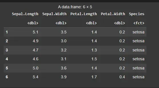
Iris Dataset

3. Splitting the Dataset into Training and Testing Sets

We need to split the dataset into two parts, training and testing. We will use 80% of the data for training and the remaining 20% for testing.

• **sample(): Randomly selects rows for the training set, ensuring that 80% of the data is used for training. R `

set.seed(42)

trainIndex <- sample(1:nrow(iris), 0.8 * nrow(iris)) trainData <- iris[trainIndex, ] testData <- iris[-trainIndex, ]

`

4. Defining the Model

We will apply the **randomForest() function to classify the species of iris plants.

• **Species ~ . : specifies that we want to predict the species based on all other variables in the dataset.
• **importance = TRUE : allows us to evaluate the importance of each feature.
• **proximity = TRUE : helps in calculating the proximity of the observations. R `

iris.rf <- randomForest(Species ~ ., data = trainData, importance = TRUE, proximity = TRUE)

`

4. Printing the Classification Model

After creating the Random Forest model, we will print the summary of the model to view its details, including the error rate and confusion matrix.

R `

print(iris.rf)

`

**Output:

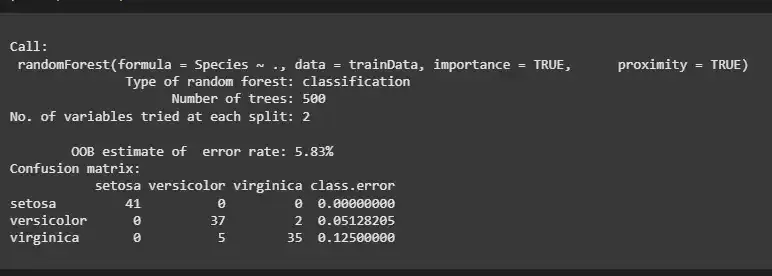
Classification Model

We can observe that

• **Type of Random Forest: The model is a classification model, meaning it is designed to predict categorical outcomes (in this case, the species of the iris plants).
• **Number of Trees: The model uses 500 decision trees to make predictions. More trees typically improve the model's accuracy by averaging the results.
• **OOB Error Rate: The Out-of-Bag (OOB) error rate is 5.83% which reflects the accuracy of the model based on data that was not used during training. A lower OOB error rate indicates better performance.

**Confusion Matrix: The confusion matrix shows the number of correct and incorrect classifications for each species.

• **Setosa: 41 correct predictions, 0 misclassifications.
• **Versicolor: 37 correct predictions, 2 misclassifications (5.13% error).
• **Virginica: 35 correct predictions, 5 misclassifications (12.5% error).

5. Making Predictions on the Test Set

Once the model is trained, we use it to make predictions on the test data.

• **predict(): This function applies the trained model to the testData to predict the species for the test set. R `

predictions <- predict(iris.rf, newdata = testData)

`

6. Plotting the Confusion Matrix (Actual vs Predicted Values)

We can evaluate the performance of our model by comparing the actual and predicted values using a confusion matrix. We create a confusion matrix using the table()function which compares the predicted values (predictions) with the actual values (testData$Species).

• **table(): Generates the confusion matrix, comparing the predicted and actual species.
• **ggplot(): Visualizes the confusion matrix using a heatmap, where the fill aesthetic represents the count of each prediction.
• **geom_tile(): Creates the heatmap tiles.
• **geom_text(): Adds the count of predictions in each tile.
• **scale_fill_gradient(): Applies a color gradient, where lower values are light blue and higher values are dark blue.
• **labs(): Adds a title and axis labels.
• **theme(): Rotates the x-axis labels for better readability. R `

confMatrix <- table(Predicted = predictions, Actual = testData$Species)

confMatrixDF <- as.data.frame(confMatrix) colnames(confMatrixDF) <- c("Predicted", "Actual", "Count")

ggplot(data = confMatrixDF, aes(x = Actual, y = Predicted, fill = Count)) + geom_tile() + geom_text(aes(label = Count), color = "white", size = 5) + scale_fill_gradient(low = "white", high = "blue") + theme_minimal() + labs(title = "Confusion Matrix", x = "Actual", y = "Predicted") + theme(axis.text.x = element_text(angle = 45, hjust = 1))

`

**Output:

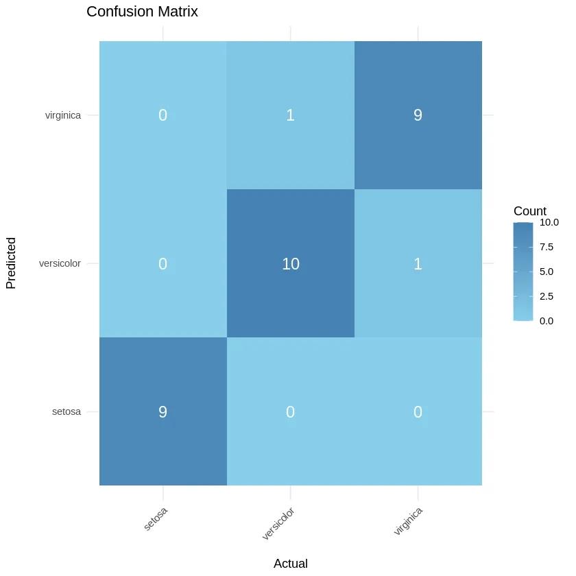
Confusion Matrix

The confusion matrix indicates the following:

• **Setosa: 9 correct predictions, 0 misclassifications.
• **Versicolor: 10 correct predictions, 1 misclassification (1 error).
• **Virginica: 9 correct predictions, 1 misclassification (1 error).

7. Plotting the Error vs Number of Trees Graph

To visualize how the error changes as we increase the number of trees, we can plot a graph showing the relationship between the error rate and the number of trees.

• **plot() : visualizes the relationship between the error rate and the number of trees in the Random Forest model. R `

plot(iris.rf)

`

**Output:

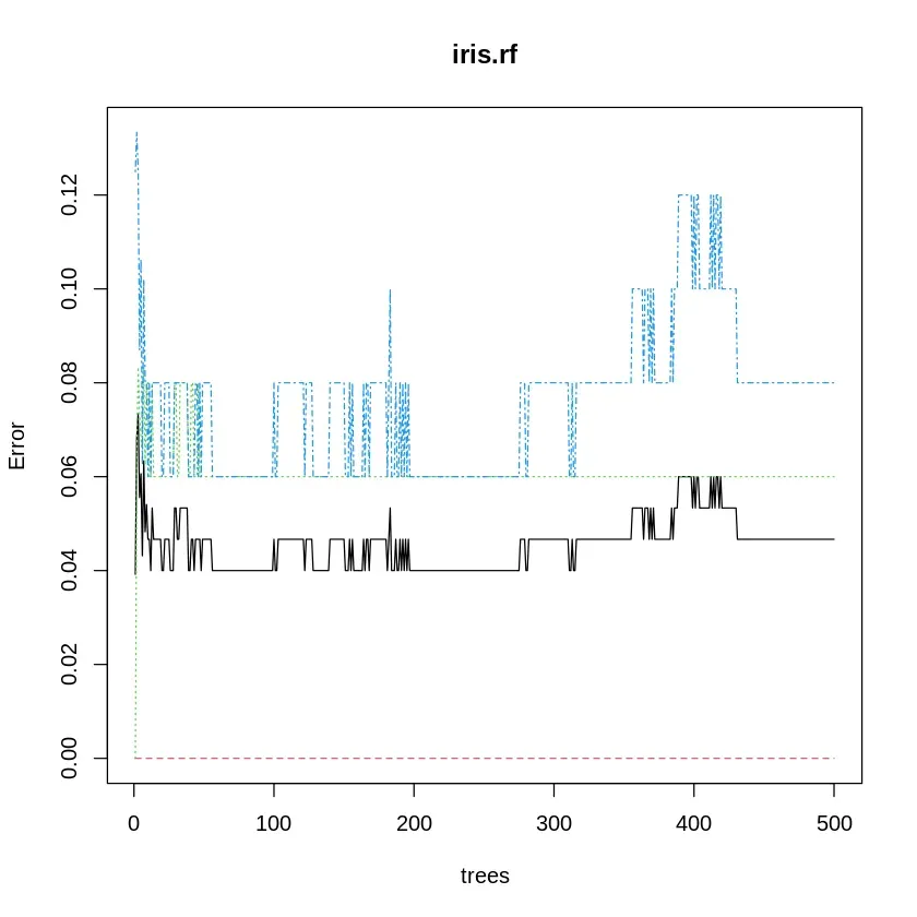
Error vs Number of Trees

As the number of trees increases, the error rate will generally decrease and stabilize. The graph helps determine the optimal number of trees to prevent overfitting while ensuring good model performance.