Random Forest Approach for Regression in R Programming (original) (raw)
Last Updated : 10 Dec, 2025
Random Forest is a supervised learning algorithm and an ensemble learning model that combines multiple decision trees to improve accuracy and reduce overfitting. By averaging the predictions of several trees, it provides more stable and robust results for both classification and regression tasks. This approach enhances the model’s ability to generalize well to unseen data.
Key Features of Random Forest
- **Aggregates Multiple Decision Trees: Combining predictions to increase model accuracy and stability.
- **Reduces Overfitting: By using multiple trees trained on different data samples, Random Forest reduces overfitting and improves generalization.
- **Handles Missing Data: Random Forest can handle missing values by averaging results from all decision trees.
- **Feature Importance: Random Forest evaluates the importance of each feature, helping identify key predictors for the target variable.
Implementation of Random Forest for Regression in R
We will train a model using the **airquality dataset in R and perform predictions on the Ozone levels based on the other features (like Solar Radiation, Wind speed and Temperature). We will also visualize the results.
1. Installing and Loading the Required Packages
We first need to install and load the **randomForest package.
R `
install.packages("randomForest")
library(randomForest)
`
2. Exploring the Dataset
We will use the **airquality dataset which contains measurements related to air quality. It includes columns like Ozone, Solar Radiation, Wind speed, Temperature, Month and Day. We will use these features to predict the Ozone levels.
R `
data("airquality") head(airquality)
`
**Output:
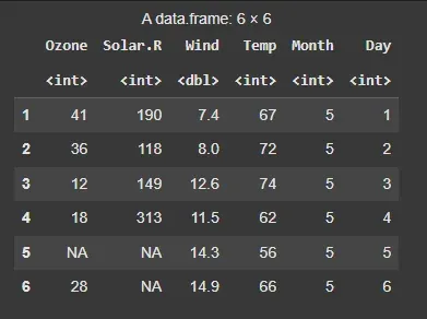
Dataset
3. Handling Missing Data
The airquality dataset has missing values in some columns. We’ll remove rows with missing values to ensure the model works correctly.
R `
airquality_clean <- na.omit(airquality)
`
4. Creating the Random Forest Model
Now we will create the Random Forest regression model to predict Ozone based on the other variables.
- **Ozone ~ . : This creates a formula for predicting the Ozone variable based on all other variables in the dataset.
- **mtry = 3: specifies that 3 variables will be randomly selected at each split in the decision trees.
- **importance = TRUE: This will calculate the importance of each feature in the regression model. R `
ozone.rf <- randomForest(Ozone ~ ., data = airquality_clean, mtry = 3, importance = TRUE)
`
5. Printing Model Results
Let’s inspect the output of the model to understand how well it performed.
R `
print(ozone.rf)
`
**Output:
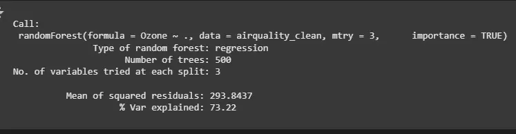
Random Forest Model
- Mean of squared residuals: Measures the error of the model’s predictions. A lower value indicates better performance.
- % Var explained: Indicates how much of the variance in the Ozone variable is explained by the model (72.43%).
6. Making Predictions
We will use the trained model to predict Ozone levels based on the features of the **airquality_clean dataset.
R `
ozone_predictions <- predict(ozone.rf, airquality_clean) op <- as.data.frame(ozone_predictions)
head(op)
`
**Output:
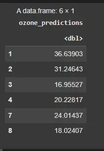
Making Predictions
7. Plotting Actual vs Predicted Values
We’ll create a plot to compare the actual Ozone values with the predicted values from the Random Forest model.
R `
plot(airquality_clean$Ozone, ozone_predictions, main = "Actual vs Predicted Ozone Levels", xlab = "Actual Ozone", ylab = "Predicted Ozone", col = "blue", pch = 19)
abline(0, 1, col = "red", lwd = 2)
`
**Output:
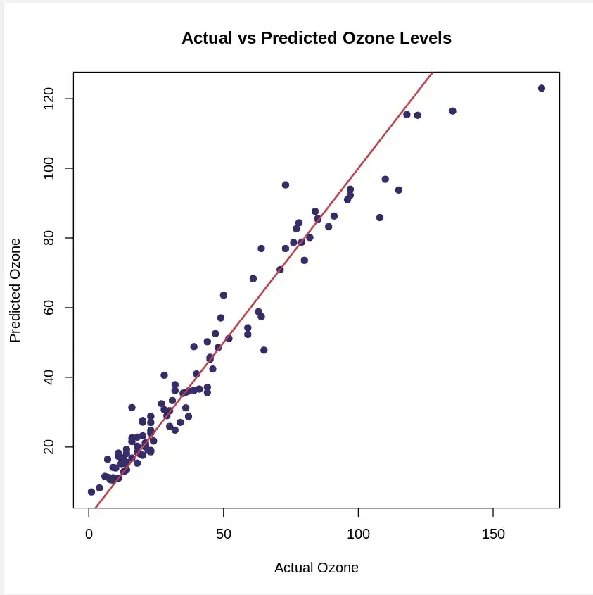
Actual vs Predicted Value
8. Calculating Feature Importance
We can also visualize the importance of each feature in predicting Ozone levels using the importance() function and **varImpPlot() function. The plot will show which features (e.g. Solar.R, Wind, Temp) are most influential in predicting the Ozone levels.
R `
importance(ozone.rf)
varImpPlot(ozone.rf)
`
**Output:
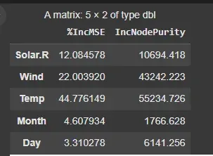
importance()
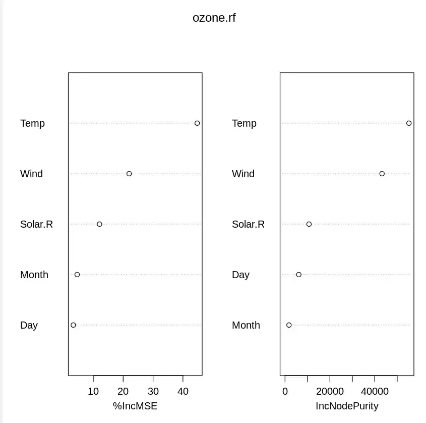
varImpPlot()
9. Plotting Error vs Number of Trees
We can also visualize how the error rate changes with the number of trees. This helps us understand the stability of the model as it learns more from the data.
R `
plot(ozone.rf)
`
Output:
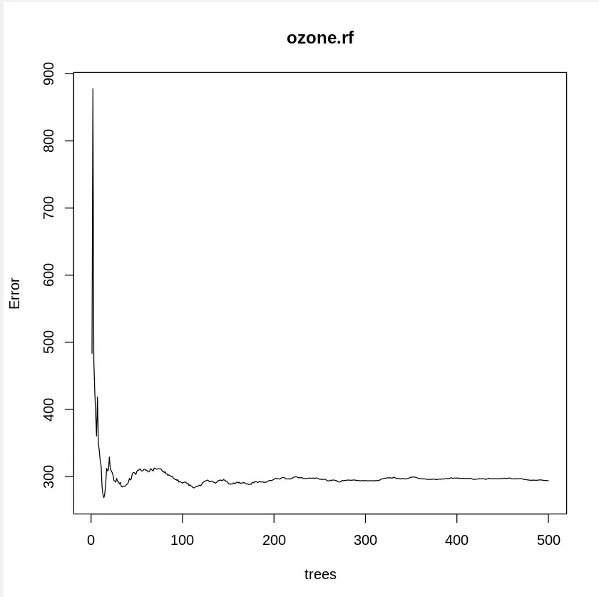
Error vs Number of Trees
The plot shows how the model’s error decreases as the number of trees increases, indicating that the model improves with more trees.
Advantages and Disadvantages of Random Forest
Advantages:
- Efficient for large datasets.
- Highly accurate, reduces bias and variance.
- Handles both categorical and continuous data effectively.
- Robust against overfitting.
Disadvantages:
- Memory-intensive and requires more resources compared to single decision trees.
- Less interpretable than individual decision trees.