Type I Error in R (original) (raw)

Last Updated : 25 Jul, 2025

A Type I error occurs when we reject a true null hypothesis. In simpler terms, it means detecting an effect or difference that doesn’t actually exist. This kind of false positive is quantified using alpha (\alpha), the pre-set significance level (commonly 0.05).

For example, in a clinical trial, if a new drug is wrongly declared effective even though it has no real impact, that’s a Type I error. This can lead to:

• Misleading conclusions from data
• Wasted resources on invalid results
• Damage to research credibility

Why Type I Errors Matter

Understanding Type I errors is important because:

• **Research Validity: False positives weaken the reliability of conclusions.
• **Resource Use: In fields like medicine, accepting ineffective treatments can waste time and harm patients.
• **Reputation Risk: Incorrect findings can hurt a researcher's or institution's credibility.

Type I Error in Hypothesis Testing

In hypothesis testing, we choose a significance level \alpha to represent our tolerance for making a Type I error. For instance, \alpha=0.05 means we're accepting a 5% chance of rejecting a true null hypothesis.

Implementation of Type I Error in R

We are estimating the Type I error rate using different techniques available in R programming language. These methods help us understand how often we may wrongly reject the null hypothesis when it is actually true.

1. Running a Simulation Approach

We are simulating multiple hypothesis tests under the null condition using a t-test and calculating the proportion of false positives.

• **alpha: Threshold used to determine statistical significance.
• **sample_size: Number of observations in each simulated sample.
• **num_simulations: Total number of t-tests performed.
• **rnorm: Generates random numbers from a normal distribution.
• **t.test: Performs a two-sample t-test to compare means.
• **p.value: Probability of observing the test result under the null hypothesis.
• **cat: Used to concatenate and display output. R `

alpha <- 0.05 sample_size <- 30 num_simulations <- 10000 false_positives <- 0

for (i in 1:num_simulations) { sample1 <- rnorm(sample_size, mean = 0, sd = 1) sample2 <- rnorm(sample_size, mean = 0, sd = 1) t_test_result <- t.test(sample1, sample2) if (t_test_result$p.value <= alpha) { false_positives <- false_positives + 1 } }

type1_error_rate <- false_positives / num_simulations cat("Type I Error Rate:", type1_error_rate)

`

**Output:

Type I Error Rate: 0.0515

2. Performing Bootstrapping for Type I Error

We are using bootstrapping to repeatedly draw samples under the null hypothesis and estimate the Type I error rate based on p-values.

• **set.seed: Ensures reproducibility of random results.
• **n: Number of observations in each resampled dataset.
• **mu: True mean under the null hypothesis.
• **alpha: Chosen significance level for testing.
• **B: Number of bootstrap samples.
• **t_test_func: Function to return the p-value from a one-sample t-test.
• **replicate: Repeats the bootstrap sampling and testing process.
• **mean: Calculates the average proportion of rejected null hypotheses. R `

set.seed(123) n <- 30 mu <- 0 alpha <- 0.05 B <- 1000

t_test_func <- function(data) { t.test(data, mu = mu)$p.value }

type_I_errors <- replicate(B, { data <- rnorm(n, mean = mu, sd = 1) t_test_func(data) })

type_I_error_rate <- mean(type_I_errors < alpha) print(type_I_error_rate)

`

**Output:

0.044

3. Running Monte Carlo Simulation for Type I Error

We are applying Monte Carlo simulation to repeatedly generate data under the null hypothesis and measure how often the null is wrongly rejected.

• **rnorm: Creates random samples from the normal distribution.
• **replicate: Performs repeated simulations to assess Type I error.
• **mean: Computes the proportion of tests that incorrectly rejected the null. R `

set.seed(123) n <- 30 mu <- 0 alpha <- 0.05 B <- 1000

t_test_func <- function(data) { t.test(data, mu = mu)$p.value < alpha }

type_I_errors <- replicate(B, { data <- rnorm(n, mean = mu, sd = 1) t_test_func(data) })

type_I_error_rate <- mean(type_I_errors) print(type_I_error_rate)

`

**Output:

0.044

4. Visualizing the Type I Error Rejection Region

We are plotting the null distribution and visually showing the rejection region where a Type I error may occur.

• **seq: Generates a sequence of values for the x-axis.
• **dnorm: Computes the normal density values for plotting.
• **plot: Draws the normal distribution curve.
• **abline: Adds a horizontal reference line to the plot.
• **polygon: Shades the rejection region on both tails of the distribution. R `

alpha <- 0.05 n <- 30 mu <- 175 sd <- 10

x <- seq(mu - 4sd, mu + 4sd, length.out = 100) y <- dnorm(x, mean = mu, sd = sd)

plot(x, y, type = "l", main = "Type I Error Visualization", xlab = "Height", ylab = "Density") abline(h = 0, col = "gray")

polygon(c(mu - qnorm(1 - alpha/2)*sd/sqrt(n), mu - qnorm(1 - alpha/2)*sd/sqrt(n), mu + qnorm(1 - alpha/2)*sd/sqrt(n), mu + qnorm(1 - alpha/2)*sd/sqrt(n)), c(0, dnorm(mu - qnorm(1 - alpha/2)*sd/sqrt(n), mu, sd), dnorm(mu + qnorm(1 - alpha/2)*sd/sqrt(n), mu, sd), 0), col = "red", density = 30, angle = 45)

`

**Output:

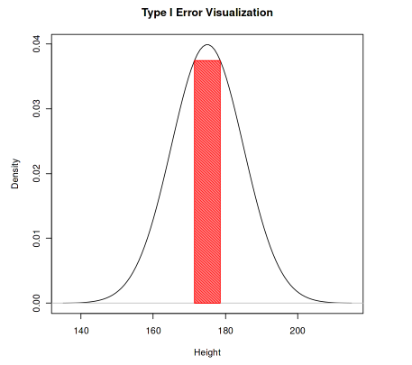
Type I Error in R

A plot showing the normal distribution curve with the rejection region shaded in red. This visual highlights where the null hypothesis would be wrongly rejected under a two-tailed test.\alpha