Discrete Fourier Transform and its Inverse using MATLAB (original) (raw)

Last Updated : 31 Jul, 2025

The Discrete Fourier Transform (DFT) and its Inverse (IDFT) are core techniques in digital signal processing. They convert signals between the time or spatial domain and the frequency domain, revealing frequency components in data. MATLAB offers useful tools for implementing and visualizing these transforms.

Mathematical Foundations

The standard equations which define how the Discrete Fourier Transform and the Inverse convert a signal from the time domain to the frequency domain and vice versa are as follows:

**DFT: The Discrete Fourier Transform (DFT) of a sequence x(n) of length N is:

X(k) = \sum_{n=0}^{N-1} x(n) \cdot e^{-j 2\pi k n / N}

Where:

• k= 0, 1, ..., N - 1
• X(k) gives the frequency-domain representation.

**IDFT: The Inverse Discrete Fourier Transform (IDFT) reconstructs the original sequence:

x(n) = \frac{1}{N} \sum_{k=0}^{N-1} X(k) \cdot e^{j 2\pi k n / N}

Where:

• n = 0, 1, ..., N-1
• x(n) is the reconstructed time-domain signal.

When we take the twiddle factors as components of a matrix, it becomes much easier to calculate the DFT and IDFT. Therefore, if our frequency-domain signal is a single-row matrix represented by X_N and the time-domain signal is also a single-row matrix represented as x_N......

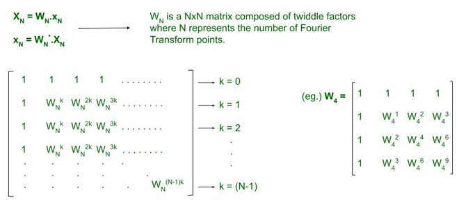
With this interpretation, all we require to do is create two arrays upon which we shall issue a matrix multiplication to obtain the output. The output matrix will always be a **Nx1 order matrix since we take a single-row matrix as our input signal (X_N or x_N). This is essentially a vector which we may transpose to a horizontal matrix for our convenience.

Step-by-Step DFT in MATLAB

1. Define the input sequence and target number of DFT points (N).
2. Zero-pad the input as needed (if length < N).
3. Build the DFT matrix using nested loops or vectorized code.
4. Multiply the DFT matrix by the input vector to compute the DFT. Matlab `

clc; xn=input('Input sequence: '); N = input('Enter the number of points: '); Xk=calcdft(xn,N); disp('DFT X(k): '); disp(Xk); mgXk = abs(Xk); phaseXk = angle(Xk); k=0:N-1; subplot (2,1,1); stem(k,mgXk); title ('DFT sequence: '); xlabel('Frequency'); ylabel('Magnitude'); subplot(2,1,2); stem(k,phaseXk); title('Phase of the DFT sequence'); xlabel('Frequency'); ylabel('Phase');

function[Xk] = calcdft(xn,N) L=length(xn); if(N<L) error('N must be greater than or equal to L!!') end x1=[xn, zeros(1,N-L)]; for k=0:1:N-1 for n=0:1:N-1 p=exp(-i2pink/N); W(k+1,n+1)=p; end end disp('Transformation matrix for DFT') disp(W); Xk=W*(x1.') end

`

**Output:

>> Input sequence: [1 4 9 16 25 36 49 64 81] >> Enter the number of points: 9

• The input sequence is zero-padded if needed to match N.
• The DFT matrix W is explicitly built using nested loops.
• The output Xk contains complex-valued frequency-domain samples.
• The code displays both the **magnitude and **phase spectrum with stem plots which are standard for discrete data.

Step-by-Step IDFT in MATLAB

1. Provide the frequency-domain sequence X(k).
2. Build the IDFT matrix using exponentials with positive sign.
3. Multiply and scale by 1/N to recover the time-domain sequence. Matlab `

clc; Xk = input('Input sequence X(k): '); xn=calcidft(Xk); N=length(xn); disp('xn'); disp(xn); n=0:N-1; stem(n,xn); xlabel('time'); ylabel('Amplitude');

function [xn] = calcidft(Xk) N=length(Xk); for k=0:1:N-1 for n=0:1:N-1 p=exp(i2pink/N); IT(k+1,n+1)=p; end end disp('Transformation Matrix for IDFT'); disp(IT); xn = (IT*(Xk.'))/N; end

`

**Output:

>> Enter the input sequence: [1 2 3 4 5 9 8 7 6 5]

• The IDFT matrix is constructed similarly but uses exp (+1i*...) to inverse the frequency components.
• The output is divided by N, as required by the mathematical formula.
• Output is plotted using stem for a clear, discrete view.