Morphogen Gradient Formation (original) (raw)
Abstract
How morphogen gradients are formed in target tissues is a key question for understanding the mechanisms of morphological patterning. Here, we review different mechanisms of morphogen gradient formation from theoretical and experimental points of view. First, a simple, comprehensive overview of the underlying biophysical principles of several mechanisms of gradient formation is provided. We then discuss the advantages and limitations of different experimental approaches to gradient formation analysis.
Morphogen concentration gradients are essential for developmental patterning. Morphogen diffusion, degradation, and endocytic transport all help to set up and maintain them.
How a multicellular organism develops from a single fertilized cell has fascinated people throughout history. By looking at chick embryos of different developmental stages, Aristotle first noted that development is characterized by growing complexity and organization of the embryo (Balme 2002). During the 19th century, two events were recognized as key in development: cell proliferation and differentiation. Driesch first noted that to form organisms with correct morphological pattern and size, these processes must be controlled at the level of the whole organism. When he separated two sea urchin blastomeres, they produced two half-sized blastula, showing that cells are potentially independent, but function together to form a whole organism (Driesch 1891, 1908). Morgan noted the polarity of organisms and that regeneration in worms occurs with different rates at different positions. This led him to postulate that regeneration phenomena are influenced by gradients of “formative substances” (Morgan 1901).
The idea that organisms are patterned by gradients of form-providing substances was explored by Boveri and Hörstadius to explain the patterning of the sea urchin embryo (Boveri 1901; Hörstadius 1935). The discovery of the Spemann organizer, i.e., a group of dorsal cells that when grafted onto the opposite ventral pole of a host gastrula induce a secondary body axis (Spemann and Mangold 1924), suggested that morphogenesis results from the action of signals that are released from localized groups of cells (“organizing centers”) to induce the differentiation of the cells around them (De Robertis 2006). Child proposed that these patterning “signals” represent metabolic gradients (Child 1941), but the mechanisms of their formation, regulation, and translation into pattern remained elusive.
In 1952, Turing showed that chemical substances, which he called morphogens (to convey the idea of “form producers”), could self-organize into spatial patterns, starting from homogenous distributions (Turing 1952). Turing’s reaction–diffusion model shows that two or more morphogens with slightly different diffusion properties that react by auto- and cross-catalyzing or inhibiting their production, can generate spatial patterns of morphogen concentration. The reaction–diffusion formalism was used to model regeneration in hydra (Turing 1952), pigmentation of fish (Kondo and Asai 1995; Kondo 2002), and snails (Meinhardt 2003).
At the same time that Turing showed that pattern can self-organize from the production, diffusion, and reaction of morphogens in all cells, the idea that morphogens are released from localized sources (“organizers” à la Spemann) and form concentration gradients was still explored. This idea was formalized by Wolpert with the French flag model for generation of positional information (Wolpert 1969). According to this model, morphogen is secreted from a group of source cells and forms a gradient of concentration in the target tissue. Different target genes are expressed above distinct concentration thresholds, i.e., at different distances to the source, hence generating a spatial pattern of gene expression (Fig. 1C).
Figure 1.

Tissue geometry and simplifications. (A) Gradients in epithelia (left) and mesenchymal tissues (right). Because of symmetry considerations, one row of cells (red outline) is representative for the whole gradient. (B) Magnified view of the red row of cells shown in A. Cells with differently colored nuclei (brown, orange, and blue) express different target genes. (C) A continuum model in which individual cells are ignored and the concentration is a function of the positions x. The morphogen activates different target genes above different concentration thresholds (brown and orange).
Experiments in the 1970s and later confirmed that tissues are patterned by morphogen gradients. Sander showed that a morphogen released from the posterior cytoplasm specifies anterioposterior position in the insect egg (Sander 1976). Chick wing bud development was explained by a morphogen gradient emanating from the zone of polarizing activity to specify digit positions (Saunders 1972; Tickle, et al. 1975; Tickle 1999). The most definitive example of a morphogen was provided with the identification of Bicoid function in the Drosophila embryo (Nüsslein-Volhard and Wieschaus 1980; Frohnhöfer and Nüsslein-Volhard 1986; Nüsslein-Volhard et al. 1987) and the visualization of its gradient by antibody staining (Driever and Nüsslein-Volhard 1988b, 1988a; reviewed in Ephrussi and St Johnston 2004). Since then, many examples of morphogen gradients acting in different organs and species have been found.
In an attempt to understand pattern formation in more depth, quantitative models of gradient formation have been developed. An early model by Crick shows that freely diffusing morphogen produced in a source cell and destroyed in a “sink” cell at a distance would produce a linear gradient in developmentally relevant timescales (Crick 1970). Today, it is known that a localized “sink” is not necessary for gradient formation: Gradients can form if all cells act as sinks and degrade morphogen, or even if morphogen is not degraded at all. Here, we review different mechanisms of gradient formation, the properties of these gradients, and the implications for patterning. We discuss the theory behind these mechanisms and the supporting experimental data.
THEORETICAL DESCRIPTIONS OF MORPHOGEN GRADIENT FORMATION
General Considerations
Crick presented his model of morphogen diffusion for a row of cells and recognized that this simplified one-dimensional scenario can easily be generalized to two- and three-dimensional tissues, e.g., epithelia or mesenchyme (Crick 1970). Because gradients are often symmetric around their source (i.e., in all directions the concentration changes the same way) (Fig. 1), the theoretical analysis is performed for one dimension.
Usually, morphogen is produced in the source and subsequently spreads in the target tissue and is degraded. Gradient formation can thus be formalized by describing the spatial and temporal changes in morphogen concentration c due to morphogen production, spreading, and degradation. When these processes are equilibrated, such that the gradient appears unchanging, it is said to have reached a steady state (Box 1).
BOX 1. General considerations.
Morphogen spreading by nondirectional movement and spatially uniform degradation can be described mathematically by an effective transport equation with an effective diffusion coefficient D [μm2/s] and effective degradation rate k [1/s]:
(Here, the concentration c [molecules/μm3] is a function of space and time, i.e., c(x, t). For simplicity, throughout the text, we write c.)
(B1.1) is a differential equation: It describes the change in morphogen concentration c over time t (∂c/∂t). It is a partial differential equation because it contains derivatives with respect to space (∂2_c_/∂x_2, in which x [μm] is the distance from the source) as well as time (∂_c/∂t). It is linear, because all terms are proportional to c. Because it contains a second derivative (∂2_c_/∂_x_2), it is called a linear partial differential equation of second order.
The first term on the right side of equation (B1.1) is a diffusion term. It describes the spreading of molecules in space due to diffusion with a diffusion coefficient D [μm2/s]. The second term is a degradation term: it describes how the concentration is reduced because of constant degradation with rate k [1/s]. (For derivation of these terms, see Box 2.)
Equation (B1.1) describes how the concentration will change in time given starting conditions. The initial condition for gradient formation in the target tissue is usually that the concentration c at time t = 0 (i.e., before the onset of morphogen production) is zero everywhere (c(x,0) = 0). A fluorescence recovery after photobleaching (FRAP) experiment, by contrast, would be characterized by a different initial condition, in which the concentration is zero only in a spatially restricted bleached area. Boundary conditions describe the behavior of molecules at the “edges” of the tissue. For instance, imagine that there is a tissue that consists of one row of cells and the first cell is the morphogen source. The target tissue abuts the source at x = 0 and has a width L [μm]. Because the source cell constantly produces and secretes molecules, at x = 0 there is a net flux (j_0 [molecules/(μm2×s)]) of molecules coming from the source. A flux of diffusing molecules is caused by a concentration difference in space (∂_c/∂x). Molecules counteract this concentration gradient by diffusing, i.e.,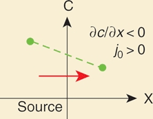
At x = L the target tissue ends and molecules bounce back, because they cannot diffuse out of the tissue (this is called a reflective boundary condition). This flattens the concentration gradient very close to the boundary, i.e., ∂c/∂x = 0, and therefore there is no net flux:
Note that in a model in which there is a spatially localized sink (Crick 1970), there is flux of molecules out of the target into the sink at x = L.
At long times (longer than the morphogen half-life) after the onset of morphogen production, the gradient approaches a steady state: the concentration does not change anymore, i.e., ∂c/∂t = 0. Consequently, the steady state equation (B1.1) does not depend on time any more, hence the solution c is a function only of x. All steady-state gradients are stable. However, it is noteworthy that not all non-steady-state gradients are unstable (see main text). The steady-state solution allows assessing the gradient properties at late developmental times, when the steady state is reached.
Steady-state solutions require that the equation parameters (D, k, and _j_0) do not depend on time. However, sometimes it is interesting to analyze effects of changing parameter values over time, e.g., temporal changes in _j_0 could indicate how a growing source will affect the gradient profile. If a parameter is changed in very small steps and after every step the gradient adjusts to the new steady state, the changes are adiabatic. When parameters change adiabatically, the gradient will always be very near the steady state. Hence, in these cases, the steady-state solution can be used to study gradient evolution over time.
Morphogen concentration changes in tissues can be described in several ways (Reeves et al. 2006). Discrete descriptions explicitly consider how each cell participates in morphogen transport and hence represent high-resolution pictures of the cellular processes underlying gradient formation, e.g., extracellular diffusion, receptor binding, internalization, recycling, and intra- and extracellular degradation. Such models are specific for the underlying transport mechanism, which can be different for different morphogens and tissues (e.g., movement by extracellular diffusion, transcytosis, and cytonemes).
Alternatively, gradient formation can be described by continuum models: low-resolution pictures in which morphogen concentration changes continuously in space and individual cells are not distinguished (Fig. 1C). In addition, instead of considering cellular and kinetic processes explicitly, they can be effectively described, e.g., random walk of molecules with an effective diffusion coefficient and effective degradation rate (Bollenbach et al. 2007). Such descriptions are simpler than discrete models and capture the essential biophysical principles that govern morphogen transport and account for gradient shape.
To illustrate different theoretical aspects of gradient formation, below we present some examples from the literature. However, we do not attempt to classify morphogens into categories: The same morphogen may use different mechanisms to form gradients in different tissues and species. As new data is gathered, models will be revised to capture gradient formation accurately in each individual case.
Gradients Formed by Diffusion
In an idealized situation, in which there is no degradation or another depleting effect, gradient formation in the target by nondirectional morphogen spreading via random walk is described by the diffusion equation, also known as Fick’s second law:
in which the rate of change of the concentration c, ∂c/∂t (at position x and time t) is proportional to the second derivative of the concentration with respect to space ∂2_c_/∂_x_2 (at x and t). The proportionality factor is the diffusion coefficient D. For derivation, see Box 2 and Berg (1993).
BOX 2. Derivation of the diffusion and degradation terms.
Imagine a cell at a distance x [µm] from the morphogen source. There is a flux of molecules into and out of the cell and molecules are not degraded. If the number of molecules that enter and leave the cell per unit time is the same, the concentration change over time in the cell is zero (∂c/∂t = 0). Conversely, if the concentration change is not zero, then there must be a change in the flux (j [molecules/(μm2×s)]) of molecules through the cell (i.e., in x):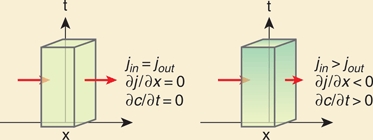
This equation is called a conservation or continuity equation: If the concentration at a certain position diminishes over time, this is accounted for by the disappearance of molecules from this position and appearance at other positions, i.e., molecules do not vanish.
A flux of diffusing molecules is caused by a concentration difference in space (∂c/∂x) (see Box 1). Molecules counteract this difference by diffusing with a diffusion coefficient D [μm2/s]:
Taking (B2.1) and (B2.2) together, we obtain
| ∂c∂t=−∂∂x(−D∂c∂x)=D∂2c∂x2∂c∂t=D∂2c∂x2 | (B2.3) |
|---|
This is called the diffusion equation.
If molecules are degraded with a constant rate k [1/s] but do not diffuse, the concentration within the cell will continuously decrease (∂c/∂t < 0). If at any time a constant percentage of the current concentration is lost, i.e., (−∂c/∂t)/c = constant = k, we can write
This is called linear degradation because ∂c/∂t is proportional to c (k itself does not depend on c). Linear degradation causes an exponential decrease of the concentration in time, i.e., c = c i e_−_kt, in which c i is the initial concentration. To verify that c = c i e_−_kt is indeed a solution, we insert it into equation (B2.4):
∂c∂t=−kc∂c∂t=∂(cie−kt)∂t=−kcie−kt=−kc
Hence c = c i e_−_kt is a valid solution of equation (B2.4).
Sometimes, instead of the degradation rate k, the half-life of molecules τ[s] is used. This is the time after which the concentration has been reduced by half:
The degradation rate is thus related to the half-life by k = ln (2)/τ.
Finally, taking diffusion and degradation together, we can write the diffusion equation with linear degradation:
Because molecules are constantly secreted from the source into the target, (which is accounted for by boundary conditions [Box 1]), and there is no depletion of molecules (no negative term in equation (1)), the concentration in the tissue constantly increases (Fig. 2A). Indeed, morphogen production and diffusion leads to the formation of Gaussian gradients that do not have steady states (Berg 1993). However, temporarily stable gradients can form in the absence of degradation, as suggested for the transcription factor Bicoid in the Drosophila embryonic syncytium (Coppey et al. 2007). Nuclear divisions increase the nuclear density in the syncytium, which in turn decreases the effective diffusivity of Bicoid. As a result, the nuclear Bicoid concentration can remain stable over several nuclear divisions (for certain parameter values), although the total concentration continuously increases (Coppey et al. 2007; Shvartsman et al. 2008).
Figure 2.

Mechanisms of gradient formation. (A–D) Steady state (solid lines) and pre-steady-state gradients (dashed lines) in the target tissue (x > 0). (Insets) Steady state solutions. The picture below each graph is a schematic view of the respective gradient formation mechanism (the respective differential equation at the bottom). (Blue circles) Nuclei, (concentric circles) degradation (darker color corresponds to higher % degradation). (A) Gradients formed by diffusion do not have a steady state: If there is a constant flux of molecules coming from the source, concentration in the target continuously increases. (B) Steady-state gradients formed by diffusion and linear degradation have exponential shape. (C) Nonlinear degradation leads to the formation of power-law gradients. (D) Power-law gradients formed by cell-lineage transport.
Developmental events often occur rapidly (e.g., the segmental patterning of the Drosophila embryo is laid down in less than 2 h), hence cell fate may not actually be determined by steady-state gradients. Indeed, it has been suggested that the Bicoid gradient is decoded before reaching a steady state (Bergmann et al. 2007; Bergmann et al. 2008). This could also be the case for target gene specification in growing tissues in which the gradient is continuously changing, as suggested for Sonic hedgehog (Shh) in neural tube patterning (Saha and Schaffer 2006; Chamberlain et al. 2008).
When cell-fate specification occurs before the gradient reaches steady state, the onset of target gene expression and the time window during which cells are competent to respond to the gradient may be important for the patterning outcome. Indeed, the duration of signaling affects the cellular response to Shh in the neural tube (Dessaud et al. 2007), Nodal in zebrafish mesoderm/endoderm induction (Hagos and Dougan 2007), and Activin in Xenopus mesoderm formation (Green and Smith 1990; Gurdon and Bourillot 2001). In addition, once target gene domains have been specified, they may continue to depend on the morphogen gradient, but also on downstream cross-interactions between different target genes, as suggested for the Drosophila gap genes (Bergmann et al. 2007). This in turn may enhance patterning robustness against fluctuating morphogen production (Bergmann et al. 2007).
Gradients Formed by Diffusion and Linear Degradation
To generate steady-state gradients, morphogens must be degraded. Unlike the scenario in which there is a localized sink, many morphogens are degraded everywhere with a degradation rate k. If the degradation rate is constant, the degraded molecules per unit time −∂c/∂t are a constant fraction (k) of the total (c), i.e., ∂c/∂t = −kc (see Box 2), and degradation is called linear.
With a linear degradation term, the diffusion equation becomes:
Gradients formed by production from a localized source, diffusion and linear degradation according to equation (2) form exponential steady-state gradients (see Box 3, Fig. 2B):
where _c_0 is the gradient amplitude, defined as the concentration at the source boundary (x = 0), and λ is the decay length, i.e., the distance to the source at which the gradient decays to a fraction of 1/e of _c_0. _c_0 and λ are related to morphogen diffusion, degradation, and production (Box 3):
BOX 3. Solution of the diffusion equation with linear degradation for the steady state.
Consider the diffusion equation with linear degradation:
Here, D(∂2_c_/∂x_2) is a diffusion term and −_kc describes morphogen removal because of degradation with a constant rate k (see Box 2).
In the steady state, ∂c/∂t = 0 and therefore D(∂2_c_/∂_x_2) − kc = 0, i.e.,
The solution for c is to be determined. In (B3.2), the second derivative of c with respect to x is proportional to +c itself. The only functions for c with this property are exponential functions. (Alternatively, one can consider sums of hyperbolic sines and cosines, which can however be written as exponentials.) Therefore, one can propose a general solution for c:
in which _c_0, _c_1, and λ are constants to be determined. To verify that (B3.3) is a solution for c, we insert c=c0e−xλ+c1e+xλ into the left side of equation (B3.2):
∂2c∂x2=kDc∂2c∂x2=(∂2∂x2(c0e−xλ+c1e+xλ))=(∂∂x(−c0λe−xλ+c1λe+xλ))=+c0λ2e−xλ+c1λ2e+xλ=1λ2(c0e−xλ+c1e+xλ)=1λ2c=kDc
This is true if
or in other words,
To determine the constants c_0 and c_1, we need two equations. We use the two boundary conditions proposed in Box 1 (equations (B1.2) and (B1.3)). Both boundary conditions involve the flux D(∂_c/∂_x). With (B3.3), the flux equals
| D∂c∂x=D∂∂x(c0e−xλ+c1e+xλ)=D(−c0λe−xλ+c1λe+xλ)=Dλ(−c0e−xλ+c1e+xλ). | (B3.5) |
|---|
At x = 0, e+xλ and e−xλ equal 1, and the flux equals the flux of molecules coming from the source (see boundary condition (B1.2)):
| D∂c∂x|x=0=−j0Dλ(c1−c0)=−j0 | (B3.6) |
|---|
At x = L, the flux should be zero (see boundary condition (B1.3))
| D∂c∂x|x=L=0Dλ(−c0e−Lλ+c1e+Lλ)=0 i.e. (−c0e−Lλ+c1e+Lλ)=0 i0e. c1=c0e−2Lλ | (B3.7) |
|---|
If we use this term for _c_1 in (B3.6),
we can solve for _c_0:
and _c_1
| c1=j0λD(e−2Lλ1−e−2Lλ). | (B3.9) |
|---|
We see that if L is much larger than λ (L ≫ λ), the second term in _c_1 becomes 0, i.e., _c_1 = 0. _c_0 simplifies to
Here, we made use of λ=D/k (B3.4). The steady state solution for the diffusion equation with linear degradation is thus
| c(x)=c0e−xλ with c0=j0Dk and λ=Dk | (B3.11) |
|---|
(in the limit of L ≫ λ).
What is the meaning of _c_0 and λ? At x = 0, c = _c_0, thus _c_0 [molecules/μm3] is the concentration at the source boundary. At x = λ, c = _c_0 _e_−1, i.e., λ [μm] is the distance to the source at which the concentration has decayed to 1/e of _c_0.
The amplitude _c_0 depends on the flux of molecules across the source boundary _j_0, diffusion D, and degradation k. λ depends on D and k of the target and is independent of source properties. The range of the gradient, defined as the position at which the concentration decreases below detection level or a target gene activation threshold, depends on both _c_0 and λ, as an increase in either will enlarge the distance at which a certain concentration occurs (Fig. 3A).
Figure 3.

Range of exponential and power-law gradients. “Range” is defined as the width of a target gene domain x*, responding to a concentration threshold c*. (A) Exponential gradients. (Left panel) A change in _c_0 (blue profile) or λ (green profile), with respect to a reference profile (black), affects the shape of the gradient; (right panel) changes in kinetic parameters D (green), k (red), and _j_0 (blue) affect the range of the gradient in different ways. Note that changing D can lead to increase or decrease in x*, depending on the concentration threshold c*. (B) Power-law gradients. (Left) The shape depends on: A (blue), x b (green), and m (magenta). Changes in either affect the range of the gradient. (Right) Changes in the kinetic parameters D, k, _j_0, and n qualitatively have similar effects on x* as corresponding effects with exponential gradients (A).
The gradients of Decapentaplegic (Dpp) and Wingless (Wg) in Drosophila imaginal discs, and Bicoid in the embryo have been analyzed considering effective diffusion and linear degradation (Gregor et al. 2007; Kicheva et al. 2007). The nondirectional spreading of Dpp has been shown using clones that ectopically express Dpp (Entchev et al. 2000). Furthermore, the kinetic parameters of Dpp spreading were measured using FRAP (Kicheva et al. 2007) and are consistent with the timescale of steady-state gradient formation (∼8 h). FRAP experiments in regions of different GFP-Dpp concentration suggest that Dpp degradation is linear. Dpp is degraded in lysosomes and has a short half-life (estimates range from ∼45 min to ∼2 h) (Entchev et al. 2000; Teleman and Cohen 2000; Kicheva et al. 2007).
The diffusion coefficient of Bicoid has also been measured by FRAP (D ∼ 0.3 µm2/s) (Gregor et al. 2007), whereas its degradation rate is unknown. A steady state is approached at times much longer than 1/k, corresponding to λ2/D for exponential gradients (Box 1, B3.4). The measured Bicoid λ (∼100 µm) and D imply that a steady state would form in >9 h, which is inconsistent with the time of syncitial embryonic development (∼2 h) (Gregor et al. 2005). Several explanations for this phenomenon were proposed: pre-steady-state decoding (Bergmann et al. 2007; Bergmann et al. 2008); contribution of nuclear dynamics to establishing a temporarily stable gradient (Coppey et al. 2007; Gregor et al. 2007); spatial and/or temporal changes of the diffusion coefficient (Gregor et al. 2007); and contribution of active transport processes (Gregor et al. 2007).
Gradients Formed by Diffusion and Nonlinear Degradation
If degradation depends on morphogen concentration, e.g., if there is a feedback mechanism (Perrimon and McMahon 1999), it is nonlinear. For instance, Hedgehog (Hh) up-regulates its receptor Patched (Ptc), which in turn restricts the Hh signaling range (Chen and Struhl 1996), most likely by causing the internalization and degradation of a higher percentage of molecules in regions of high Hh concentration (Eldar et al. 2003). Thus, Hh enhances its own degradation. Another example is Wg degradation in the Drosophila embryo, which is accelerated by spatially inhomogeneous epidermal growth factor receptor signaling (Dubois et al. 2001).
If degradation is nonlinear, the degradation rate k is a function k(c) of the concentration:
Self-enhanced degradation is a special case of nonlinear degradation:
Thus, at higher concentrations, the degradation rate will be higher. The magnitude of degradation self-enhancement depends on the exponent n and the factor k*. The diffusion equation with nonlinear degradation becomes:
and in the special case:
Part of the analysis of equation (8) (by Eldar et al. 2003) is presented below. The steady-state solution:
shows that the concentration is proportional to 1/x m, hence this type of gradient is called a power-law gradient (Fig. 2C). Its shape is determined by the parameters A, _x_b, and m (Fig. 3B). What do these parameters mean?
For comparison with exponential gradients, the amplitude and decay length-scale of power-law gradients are given by the following equations:
| c0=Axbm and λs=x+xbm. | (10) |
|---|
Note that in contrast to exponential gradients, in which the concentration decays by the same percentage at each position, power-law gradients decay fast close to the source and more slowly at a distance, i.e., their decay length-scale λs is position-dependent and reflects the local steepness of the gradient.
The parameters A, _x_b, and m are related to the kinetic parameters of morphogen spreading, D, k, and _j_0 (Eldar et al. 2003):
| m=2n−1, A=(m(m+1)Dk∗)1n−1,xb=(mADj0)n−1n+1 | (11) |
|---|
The value of m determines the steepness of the gradient: If self-enhancement of degradation is very pronounced (high value of n, hence low value of m), a higher percentage of molecules is degraded closer to the source and the gradient is less steep. The parameter _x_b is inversely related to _j_0: If _j_0 increases, for instance because the source is growing, _x_b will become smaller and the gradient profile will be spatially shifted in x: Its range will increase (Fig. 3B). For very large values of _j_0, x b approaches zero, hence the gradient reaches a limiting profile:
which is independent of _j_0, and consequently robust with respect to changes in _j_0 (Eldar et al. 2003). This robustness is a key property that distinguishes power-law from exponential gradients. Equation (4) shows that the amplitude of exponential gradients is proportional to _j_0 and there is no limiting profile as for power-law gradients. Thus, provided that all other parameters are constant, a change in morphogen production will cause a proportional increase in the amplitude of an exponential gradient, which will lead to proportional increase of the concentration for all positions x. In contrast, in a power-law gradient, higher production and therefore higher morphogen concentration will also cause higher degradation (6). Thus, the effective increase in concentration will be smaller compared with exponential gradients, where such feedback between ligand concentration and degradation does not occur.
Nonlinear degradation does not necessarily need to follow equation (6). For instance, models of gradient formation by transcytosis, such as the Dpp gradient in the Drosophila wing disc, show that, in this scenario, both degradation and diffusion depend on concentration via more complex nonlinear functions that include trafficking rates, receptor binding, etc. (Bollenbach et al. 2005; Bollenbach et al. 2007). However, nonlinear diffusion and degradation of Dpp have not been experimentally observed (Kicheva et al. 2007), possibly because, for small ligand concentrations, D and k become concentration-independent (Bollenbach et al. 2007). Thus, gradients formed by transcytosis may be indistinguishable from exponential gradients.
Other Types of “Diffusion”
Effective diffusion models capture nondirectional morphogen spreading (Gregor et al. 2005; Kicheva et al. 2007). So far, no experimental evidence for spreading with directional bias has been found, although it has been theoretically considered: For example, transport by endocytosis and recycling in polarized cells may be directional because of inhomogeneous receptor localization, making it more likely that internalization or externalization of vesicles occurs in a certain place (Bollenbach et al. 2007). In this case, morphogen molecules move by random walk, but endogenous conditions make transport directional. This can be described by regular diffusion plus a drift term, describing molecules moving with velocity v in a certain direction (Bollenbach et al. 2007). A mechanism based on diffusion with drift and linear degradation leads to exponential steady-state gradients, in which the decay length is stretched or compressed depending on the drift direction.
A different kind of directional transport is active transport, e.g., vesicle movement on microtubules. Active transport may be nondirectional, but it cannot be described by the diffusion equation, because it invokes forces. The mean square displacement of freely diffusing molecules is linearly related to time, however, for actively transported molecules, this relationship is nonlinear (Berg 1993). This is also true, for example, for molecules that are caged in polymer networks and thus do not diffuse freely (Caspi et al. 2002). Such phenomena can be described by anomalous diffusion models, which lead to the formation of exponential gradients (Hornung et al. 2005).
Gradients Formed by Cell Lineage Transport
Contrary to the notion that morphogens must be secreted and diffuse in target tissues, it is possible to generate gradients of nonsecreted molecules just by cell growth and division (Fig. 2D). For instance, fgf8 mRNA forms a gradient during polarized growth of the vertebrate anterioposterior axis (Dubrulle and Pourquié 2004). fgf8 mRNA is expressed in the posterior-most part of the presomitic mesoderm. As cells divide and move out of the mRNA expression domain, they transport and dilute the fgf8 mRNA they contain, thus generating a gradient (Dubrulle and Pourquié 2004). The formation of a hoxd13 mRNA gradient in the developing vertebrate limb proceeds in a similar manner and has been analyzed with a discrete model (Ibañes et al. 2006). The effect studied with a continuum description of wing disc growth on Dpp has been studied with a continuum description (Baker and Maini 2006). Here, we discuss a simplified continuum model that describes gradient formation for nonsecreted molecules.
Imagine a tissue that grows exponentially and continuously. A cell can be considered a “volume element” of the tissue. Concentration is inversely proportional to volume, hence if a cell grows exponentially with a constant rate k_g [1/s], the concentration of molecules in the cell will decrease exponentially with the same rate k_g. Thus, the decrease in concentration per unit time −∂_c/∂_t will be proportional to the concentration c with a proportionality factor k_g, i.e., ∂_c/∂t = −k g c. This is called dilution of the concentration because of growth. In addition, when cells grow and divide, they transport the morphogen they contain through the tissue (Fig. 2D). There must therefore be a drift term that describes this movement (Baker and Maini 2006).
If the source width w [µm] is kept fixed, i.e., source cells that divide and cross the source boundary stop producing, cells in the target will move with a velocity k x (x + w) [μm/s]. Here, k x [1/s] is the tissue expansion rate (for tissues growing only in x, k x = k g) (Bittig et al. 2008). Cells far away from the source (large values of x) move faster than cells closer to the source, because they are pushed by more cells. The drift of molecules along x due to this movement of cells is then given by −k x(x + w) ∂c/∂x.
Gradient formation due to exponential tissue growth can thus be described by:
| ∂c∂t=−kgc−kx(x+w)∂c∂x. | (13) |
|---|
The steady-state solution:
is a _power_-law gradient, in which ζ = k g/k x depends on the tissue dimensionality (for one-dimensional tissues ζ = 1, for higher dimensions ζ > 1) (Fig. 2D) (Bittig et al. 2008). For a boundary condition that imposes a constant concentration in the source (c source), B = c source _w_ζ (as there is no diffusion, flux boundary conditions are not applicable).
Many gradients form in growing tissues and thus dilution and drift effects contribute to gradient formation. However, if growth is much slower than the turnover of a diffusion–degradation gradient, these effects might be negligible. Finally, if a gradient of nonsecreted molecules (e.g., fgf8 mRNA) is the source of morphogen (e.g., the secreted Fgf8 protein), then the formation of the protein gradient is characterized by the fact that (1) source and target cells are the same and (2) production in the tissue is graded. It is noteworthy that these two phenomena are also partially true for gradients formed by diffusion and degradation, even if the contribution of tissue growth to gradient formation is negligible. In the cases discussed, e.g., Dpp, Wg, etc., source and target are spatially distinct domains, but signaling and growth occurs in both, and morphogen production in the source may be graded.
Fine-tuning Gradient Shape
While spreading in tissues, all morphogens interact with molecules such as receptors, extracellular matrix components, inhibitors, etc., that affect gradient shape. In effective models, morphogen–modulator interactions may be part of the effective description. For example, when receptor concentrations are not limiting, Dpp-receptor interactions will affect the absolute values of the effective diffusion coefficient and degradation rate, but morphogen kinetics is still accurately described (within the boundaries of experimental error) by diffusion and linear degradation without explicitly considering receptor binding (Bollenbach et al. 2007).
Prominent gradient modulators are heparan sulfate proteoglycans (HSPGs), such as Dally and Dally-like protein, which bind to and affect the diffusion of Dpp, Wg, and Hh (Belenkaya et al. 2004; Han et al. 2004; Takei et al. 2004; Han et al. 2005). Ligand-receptor interactions shape the Hh gradient: The receptor Ptc sequesters Hh and restricts Hh signaling range, hence loss of ptc function causes Hh target gene domain expansion (Chen and Struhl 1996). Secreted inhibitors, receptors, or proteases, also affect morphogen gradients. For instance, the gradient of activated Spätzle in the Drosophila embryo is formed by a localized proteolytic cleavage of the Spätzle precursor by the Easter protease (DeLotto and DeLotto 1998; LeMosy 2006). The cleaved amino-terminal part of Spätzle could function as an Easter-inhibitor, thus contributing to gradient shape (reviewed in Moussian and Roth 2005). A secreted receptor, Frz-b, binds directly to XWnt8 and shapes the anterioposterior Wnt gradient in early Xenopus embryos (Leyns et al. 1997; Wang et al. 1997). The secreted inhibitors Noggin and Chordin bind to BMP-4 and transport it, thus shaping its gradient (Jones and Smith 1998).
What is the advantage of interactions with gradient modulators? Modulators are important for generating signaling activity gradients and their interpretation. In addition, morphogen–modulator interactions may make gradients more robust. For example, robustness of the Dpp activity gradient to changes in gene dosage in the Drosophila embryo is achieved through interaction of Dpp, Screw, and the inhibitor Sog (Eldar et al. 2002). In addition, in Xenopus embryos, a vertebrate-specific feedback repression mechanism allows the homologous BMP gradient to scale with tissue size (Ben-Zvi et al. 2008). Gradient scaling with tissue size implies that pattern also scales. For example, the Bicoid gradient range seems to change proportionally in differently sized embryos of different species and so does the domain of the target gene hunchback (Gregor et al. 2008). However, when Bicoid proteins of dipterans with larger embryos are expressed in Drosophila, they form gradients with the Drosophila decay length, suggesting that embryo-specific factors modulate Bicoid gradient shape in different species and contribute to scaling (Gregor et al. 2008).
EXPERIMENTAL MEASUREMENTS OF MORPHOGEN GRADIENTS
Target Gene Expression Domains: The Range of a Morphogen Gradient
The observations that target genes are expressed in nested domains and their widths change on gene dosage alterations have been used to show the existence of morphogen gradients (Struhl et al. 1989; Tickle 1999; Gurdon and Bourillot 2001; Green 2002; Affolter and Basler 2007). Changes of target gene expression domains are useful to infer properties of the morphogen gradient, especially when it cannot be directly visualized. For example, overexpression of dlp in the Drosophila wing disc expands the expression domains of Dpp and Wg target genes, suggesting that dlp enhances the effective diffusion of morphogens (Belenkaya et al. 2004; Han et al. 2005).
The shape of exponential gradients is defined by _c_0 and λ, which in turn depend on the diffusion coefficient D, degradation rate k, and the flux _j_0 (equation 4). The gradient range changes if _c_0, λ, or both change (Fig. 3A). If D increases, _c_0 decreases, but λ increases (Fig. 3A), and the expression domain of high-threshold target genes may shrink, while the domain of low-threshold target genes may expand. Thus, interpreting experimental results based on a single target gene range may be ambiguous. Consideration of two target gene domains circumvents this problem: The difference or the ratio of the two compared with wild-type allow to distinguish between possible causes. The same reasoning can be applied to power-law gradients (Fig. 3B).
For instance, when Reggie1, a membrane microdomain component, is overexpressed in Drosophila wing discs, the range of high-threshold Wg target genes decreases, whereas low-threshold targets expand (Katanaev et al. 2008). This implies that Reggie1 increases the effective diffusion coefficient of Wg, causing decreased _c_0 and increased λ (Fig. 3A). Reggie1 expression only in the source should decrease _c_0 (as Reggie1 increases diffusion in the source), but not change λ, which depends only on diffusion and degradation in the target. Thus, all target gene domains should shrink. Indeed, the range of high threshold targets is reduced (Katanaev et al. 2008). However, the Wg gradient is “broadened,” suggesting λ is increased. This could mean that Reggie1 modifies the Wg protein in the source, thus altering also its diffusion properties in the target.
Finally, gradient range is a readout of signaling activity. Hence, even if diffusion, degradation, and source properties are unperturbed, the range can change if downstream signaling is modified. For instance, the sumoylation of Medea, a Dpp signaling effector, restricts the Dpp signaling range in the Drosophila embryo (Miles et al. 2008).
Immunostainings and GFP–morphogen Fusions: Measuring Absolute Concentrations
To determine morphogen gradient shape directly, morphogens can be visualized by immunostainings or green fluorescent protein (GFP)–morphogen fusions. For a quantitative description, imaging conditions have to be such that fluorescence intensity (FI) is linearly proportional to concentration. This linearity can be verified with (1) a stepwise photobleaching assay (Kicheva et al. 2007), (2) FI calibration using recombinant GFP solutions with defined concentrations (Piston et al. 1999; Gregor et al. 2007; Kicheva et al. 2007), and (3) FI calibration using rotavirus-like particles tagged with a known number of GFP (Rink et al. 2005; Kicheva et al. 2007). FI from immunostainings can also be calibrated to concentration (Gregor et al. 2007). This is useful to test if the GFP-fusion protein forms the same gradient as the endogenous protein and ensures that GFP-fusion specific properties (e.g., diffusion, degradation, and folding) do not change gradient shape. Unspecific background FI should be considered in calibration procedures.
Once linear imaging is established, it is possible to determine the detection sensitivity: the percentage of molecules that are reliably detectable above background. The background FI can be measured in a control sample that does not express the GFP–morphogen fusion. In this case, any signal is caused by autofluorescence and detection noise, which is characterized by a Poisson distribution, i.e., its standard deviation (SD) is equal to the square root of the mean FI. Any signal beyond two SDs of this noise can be considered significantly higher than the noise level. The detection sensitivity is thus:
| detection sensitivity=1−2SDnoiseFIsignal−FInoise. | (15) |
|---|
Using this approach, the detection sensitivity for GFP-Dpp in the wing disc was estimated to be ∼98% in a region of interest (ROI) of 89 × 103 pixels (Kicheva et al. 2007).
Note that ROI size affects the FI value (the bigger the ROI, the more counts per ROI) and hence the detection sensitivity, because in a Poisson distribution the SD is a smaller percentage of the mean for higher mean values. Thus, for a background image with 10 counts/pixel on average, for a small 10 pixel ROI, FI/ROI = 100 and SD = 10. For a larger ROI of 100 pixels, FI/ROI = 1000 and SD = 32. If the signal is 20 counts/pixel on average, then in the small ROI the detection sensitivity is 1−(2×10)/(200−100) = 0.80 = 80%. In the large ROI, it is 1−(2 × 32)/(2000−1000) = 0.94 = 94%.
To analyze the gradient range, the FI should not be normalized, because the range depends on both _c_0 and λ. Normalization to the amplitude can be applied when the analysis focuses on the decay length. This was used to study the fluctuations of Dpp gradient shape in the Drosophila wing disc while ignoring global variations in production rate between different animals (Bollenbach et al. 2008). Morphogen gradients can also be normalized to the tissue length L. In this case, positions and decay lengths are measured as fractions of tissue length: X = (x/L) and Λ = λ/L, respectively (see also Reeves et al. 2006). Interestingly, Λ of the Bicoid gradient is conserved among dipteran species (Gregor et al. 2005; Gregor et al. 2008), suggesting that the Bicoid gradient accounts for the scaling of target gene positions in different species. It should be noted, however, that the gradient range (e.g., target gene domains) does not scale with size unless _c_0/c* is also constant (Fig. 3).
GFP–morphogen fusions represent the total morphogen pool, rather than the fraction that is actively signaling. However, the signaling pool is not static—all molecules dynamically exchange. Thus, studies of gradient formation, rather than interpretation, consider the total morphogen pool. Nevertheless, extra- and intracellular pools can be distinguished. For instance, intracellular compartments (e.g., endosomes) can be recognized by coimmunostainings or with specific particle-recognition software. In turn, extracellular immunostaining (Strigini and Cohen 2000) shows the amount of free or receptor-bound extracellular molecules. FRAP experiments can also provide clues about different morphogen pools: ∼60% of GFP-Dpp FI does not recover in a 1-h experiment, hence there is a fraction of “immobile” morphogens (Kicheva et al. 2007). This fraction is bigger than the estimated extracellular GFP-Dpp (∼15%). Intracellular molecules in target cells may signal, recycle, or be sent to degradation. As GFP fluorescence is very low in acidic pH environment (Patterson et al. 1997), molecules in late endosomes and lysosomes may not be efficiently detected, suggesting that the “immobile” GFP-Dpp fraction may constitute an intracellular signaling pool. Direct analysis of a signaling pool would however require the use of biosensors or other signaling activity reporters.
Clonal Analysis: Dissecting the Function of Genes Involved in Morphogen Transport
The generation of mutant clones in a wild-type tissue is a powerful tool to assess the functions of genes involved in morphogen gradient formation, because wild-type and mutant tissue are juxtaposed and autonomous, and nonautonomous effects can be distinguished. For example, it was analyzed how the Dpp gradient or its target genes are affected by clones that lack or overexpress its receptor (Nellen et al. 1996), proteins important for Dpp endocytosis (Entchev et al. 2000), or HSPGs (Belenkaya et al. 2004). Eldar and Barkai (2005) determined the theoretical morphogen profile in the clone vicinity if either of three properties is changed within the clone: diffusion, degradation, or the binding of morphogen molecules to immobile elements, e.g., receptors. They found that changes in morphogen levels in the clone, as well as the transient or permanent appearance of reduced or increased concentration in the clone vicinity (called “shadow” and “antishadow” respectively) allow determination of which parameter is affected.
Mosaic overexpression of the Wg receptor DFz2 in Drosophila wing discs causes higher Wg levels within clones, but also nonautonomously, suggesting a function of DFz2 in Wg stabilization, rather than diffusion or “trapping” (Cadigan et al. 1998; Eldar and Barkai 2005). In clones deficient for HSPGs or proteins required for HSPG biosynthesis, morphogen accumulates in front of the clone and a permanent shadow is formed behind it (Belenkaya et al. 2004; Takei et al. 2004). This can be attributed to decreased morphogen diffusion (Eldar and Barkai 2005). Clones mutant for a temperature-sensitive dynamin allele (shibire ts), were used to determine the role of endocytosis for Dpp gradient formation in the Drosophila wing disc (Entchev et al. 2000). On shift to the restrictive temperature (34°C), endocytosis was blocked in the clone and GFP-Dpp expression in the source started. The mutant clone was thus confronted with a propagation front of GFP-Dpp that could be monitored in and around the clone pre-steady state. Shadows, which become less pronounced in steady-state conditions, were observed behind the clone (Entchev et al. 2000). This is consistent with reduced effective diffusion of Dpp (Kruse et al. 2004).
Off-steady-state Analysis of Morphogen Kinetics
Morphogen gradient shape is determined by the kinetic parameters D, k, and _j_0 (Kicheva et al. 2007; Kicheva and González-Gaitán 2008). Different combinations of parameter values can produce the same steady-state shape and similar shapes can result from different cellular transport mechanisms, hence it is important to measure the kinetic parameters of morphogen movement. This can be performed by in vivo imaging in conditions in which the steady state is perturbed.
A prominent method for kinetic analysis is FRAP, which has been used in short timescale experiments (several minutes) to measure the fluorescence recoveries of GFP-tagged proteins in cells (Lippincott-Schwartz et al. 2003), as well as on long timescales (1 h) to study GFP-morphogen kinetics in tissues (Kicheva et al. 2007). On long timescales, the FI recovery in a bleached region depends on morphogen production, diffusion, and degradation (Fig. 4). By fitting the measured fluorescence recovery to the theoretical function obtained by solving the diffusion equation with production and linear degradation, D, k, and _j_0 for GFP-Dpp and GFP-Wg were determined in Drosophila wing discs (Kicheva et al. 2007). The diffusion coefficient of Bicoid-GFP in the Drosophila embryo was also determined using FRAP (Gregor et al. 2007). Bicoid-GFP recovery in the cortical cytoplasm was fast (∼60 s, in contrast to 1 h for GFP-Dpp in the wing disc) and the diffusion coefficient was derived from fitting the data to a 3-dimensional diffusion model without degradation.
Figure 4.

FRAP in epithelia. (A) (top) A vertical stripe next to the source of a two-dimensional epithelial sheet is bleached. Recovery of fluorescence is measured in the bleached stripe (red rectangle). In the adjacent region (dashed rectangle), there is loss of fluorescence (FLIP). (bottom) Theoretical recovery curves for the red and dashed regions in the top panel, depending on the spreading mechanism (diffusion and degradation [_middle_] vs. anomalous diffusion [_bottom_]). The double logarithmic plot (A, bottom) allows to distinguish the time-scales of recovery for different mechanisms. Recovery by anomalous diffusion (dashed red line) has a bigger initial slope of recovery than regular diffusion with linear or nonlinear degradation (solid red lines), respectively, in which the initial slope of recovery is close to 0.5 (dotted black line). (B) (top) A stripe perpendicular to the source is bleached. Recovery is measured in four regions at different distances to the source. Qualitative features of the recovery curves allow distinguishing between underlying mechanisms (B, center and bottom). For instance, in diffusion with linear degradation (B, center), the difference between FI recovery in two different regions continuously increases (arrows), whereas in diffusion with nonlinear degradation (B, bottom), it increases and then decreases (arrows). Depending on endogenous parameter values and experimental noise, this effect may be hard to distinguish in an experiment.
In some instances, FRAP recoveries can be used to test the underlying mechanisms. For example, anomalous and “Fickian” diffusion can be distinguished by FRAP, because the time-dependence of recovery is different for the two mechanisms (Fig. 4A) (Hornung et al. 2005). Directional and nondirectional spreading can be distinguished by photobleaching regions with different geometries or by photoactivation experiments. Bleaching regions at different distances to the source and comparing the parameter values in each case shows whether diffusion and degradation are linear. Alternatively, a stripe perpendicular to the source can be bleached and the fluorescence recovery measured in squares at different distances to the source (Fig. 4B) (Kicheva et al. 2007). The FI recovery is simultaneously fitted for all squares, imposing D, k, _j_0, and the immobile fraction to be the same for each square. If morphogen degradation were nonlinear (i.e., different closer to the source than far away), such a fit should not perform well (Fig. 4B).
FRAP has also been used to analyze the kinetics of morphogen signaling effectors that form gradients of signaling activity. For example, studies of the phosphorylation and nucleocytoplasmic shuttling of Mad, an effector of Dpp signaling, in cells (Schmierer et al. 2008) and in the Drosophila neuromuscular junction (Dudu et al. 2006) suggested that nuclear import, export, and oligodimerization are important for nuclear Mad levels. Determination of the kinetics of the Dorsal transcription factor, which forms a signaling activity gradient in Drosophila embryos (DeLotto et al. 2007) confirmed that Dorsal is actively shuttling into and out of all nuclei, independent of concentration. Complementary to FRAP, fluorescence loss in photo-bleaching (FLIP) experiments provide kinetic information about molecules in the nonbleached regions. Continuous bleaching of a region leads to loss of FI in adjacent regions caused by diffusion of molecules into the bleached area (Fig. 4A). FLIP of Dorsal-GFP in the Drosophila embryo showed that the syncitial cytoplasm is partially compartmentalized (DeLotto et al. 2007).
CONCLUDING REMARKS
The experimental and theoretical analysis of the formation of morphogen gradients allowed to focus attention on the key issues, on the important parameters that needed to be measured, and prompted efforts towards developing assays to assess them. The relative success of the strategy stemmed from performing the analysis of the system in a top-down approach: parameters (diffusion, degradation, etc.) are measured without a molecular and cell biological depth. The advantage of such a simple approach is that it avoids the consideration of too detailed mechanisms, in which using too many equations and parameters makes any model plausible: Everything is possible in Granada.
In contrast, mutant analysis revealed the importance of the underlying cell biology and the different molecules necessary to produce, move, and degrade morphogens. In the future, progress will derive from a similar type of physical, theoretical, and experimental approach at the cellular and subcellular levels: How morphogens and their receptors are moving inside cells and at the extracellular matrix.
ACKNOWLEDGMENTS
Ortrud Wartlick and Anna Kicheva contributed equally to this work.
Footnotes
Editors: James Briscoe, Peter Lawrence, and Jean-Paul Vincent
Additional Perspectives on Generation and Interpretation of Morphogen Gradients available at www.cshperspectives.org
REFERENCES
- Affolter M, Basler K 2007. The decapentaplegic morphogen gradient: From pattern formation to growth regulation. Nat Rev Genet 8:663–674 [DOI] [PubMed] [Google Scholar]
- Baker RE, Maini PK 2006. A mechanism for morphogen-controlled domain growth. J Math Biol 54:597–622 [DOI] [PubMed] [Google Scholar]
- Balme DM, ed. 2002. Aristotle: Historia animalium Cambridge University Press, Cambridge [Google Scholar]
- Belenkaya TY, Han C, Yan D, Opoka RJ, Khodoun M, Liu H, Lin X 2004. Drosophila Dpp morphogen movement is independent of dynamin-mediated endocytosis but regulated by the glypican members of heparan sulfate proteoglycans. Cell 119:231–244 [DOI] [PubMed] [Google Scholar]
- Ben-Zvi D, Shilo BZ, Fainsod A, Barkai N 2008. Scaling of the BMP activation gradient in Xenopus embryos. Nature 453:1205–1211 [DOI] [PubMed] [Google Scholar]
- Berg HC 1993. Random walks in biology Princeton University Press, Princeton [Google Scholar]
- Bergmann S, Sandler O, Sberro H, Shnider S, Schejter E, Shilo B-Z, Barkai N 2007. Pre-steady-state decoding of the Bicoid morphogen gradient. PLoS Biol 5:e46. [DOI] [PMC free article] [PubMed] [Google Scholar]
- Bergmann S, Tamari Z, Schejter E, Shilo B-Z, Barkai N 2008. Re-examining the stability of the Bicoid morphogen gradient. Cell 132:15–17; author reply 17–18 [DOI] [PubMed] [Google Scholar]
- Bittig T, Wartlick O, Kicheva A, González-Gaitán M, Jülicher F 2008. Dynamics of tissue growth with oriented cell division. New J Phys 10:063001 [Google Scholar]
- Bollenbach T, Kruse K, Pantazis P, González-Gaitán M, Jülicher F 2005. Robust formation of morphogen gradients. Phys Rev Lett 94:018103. [DOI] [PubMed] [Google Scholar]
- Bollenbach T, Kruse K, Pantazis P, González-Gaitán M, Jülicher F 2007. Morphogen transport in epithelia. Phys Rev E 75:011901. [DOI] [PubMed] [Google Scholar]
- Bollenbach TM, Pantazis P, Kicheva AK, Bökel C, González-Gaitán M, Jülicher F 2008. Precision of the Dpp gradient. Development 135:1137–1146 [DOI] [PubMed] [Google Scholar]
- Boveri T 1901. Die polarität von ovocyte, ei, und larve des strongylocentrus lividus. Zool Jahrb Abt Anat Ont Thi 14:384 [Google Scholar]
- Cadigan KM, Fish MP, Rulifson EJ, Nusse R 1998. Wingless repression of Drosophila frizzled 2 expression shapes the wingless morphogen gradient in the wing. Cell 93:767–777 [DOI] [PubMed] [Google Scholar]
- Caspi A, Granek R, Elbaum M 2002. Diffusion and directed motion in cellular transport. Phys Rev E Stat Nonlin Soft Matter Phys 66:011916. [DOI] [PubMed] [Google Scholar]
- Chamberlain CE, Jeong J, Guo C, Allen BL, McMahon AP 2008. Notochord-derived Shh concentrates in close association with the apically positioned basal body in neural target cells and forms a dynamic gradient during neural patterning. Development 135:1097–1106 [DOI] [PubMed] [Google Scholar]
- Chen Y, Struhl G 1996. Dual roles for patched in sequestering and transducing hedgehog. Cell 87:553–563 [DOI] [PubMed] [Google Scholar]
- Child CM 1941. Patterns and problems of development Chicago University Press, Chicago [Google Scholar]
- Coppey M, Berezhkovskii AM, Kim Y, Boettiger AN, Shvartsman SY 2007. Modeling the bicoid gradient: Diffusion and reversible nuclear trapping of a stable protein. Dev Biol 312:623–630 [DOI] [PMC free article] [PubMed] [Google Scholar]
- Crick F 1970. Diffusion in embryogenesis. Nature 225:420–425 [DOI] [PubMed] [Google Scholar]
- De Robertis EM 2006. Spemann’s organizer and self-regulation in amphibian embryos. Nat Rev Mol Cell Biol 7:296–302 [DOI] [PMC free article] [PubMed] [Google Scholar]
- DeLotto Y, DeLotto R 1998. Proteolytic processing of the Drosophila Spätzle protein by Easter generates a dimeric NGF-like molecule with ventralising activity. Mech Dev 72:141–148 [DOI] [PubMed] [Google Scholar]
- DeLotto R, DeLotto Y, Steward R, Lippincott-Schwartz J 2007. Nucleocytoplasmic shuttling mediates the dynamic maintenance of nuclear dorsal levels during Drosophila embryogenesis. Development 134:4233–4241 [DOI] [PubMed] [Google Scholar]
- Dessaud E, Yang LL, Hill K, Cox B, Ulloa F, Ribeiro A, Mynett A, Novitch BG, Briscoe J 2007. Interpretation of the sonic hedgehog morphogen gradient by a temporal adaptation mechanism. Nature 450:717–720 [DOI] [PubMed] [Google Scholar]
- Driesch H 1891. Entwicklungsmechanische studien, i. Der werth der beiden ersten furchungszellen in der echinodermentwicklung. Experimentelle erzeugen von theil—und doppelbildung. Z Wiss Zool 53:160–178 [Google Scholar]
- Driesch H 1908. The science and philosophy of the organism Adam and Charles Black, London [Google Scholar]
- Driever W, Nüsslein-Volhard C 1988a. The bicoid protein determines position in the Drosophila embryo in a concentration-dependent manner. Cell 54:95–104 [DOI] [PubMed] [Google Scholar]
- Driever W, Nüsslein-Volhard C 1988b. A gradient of bicoid protein in Drosophila embryos. Cell 54:83–93 [DOI] [PubMed] [Google Scholar]
- Dubois L, Lecourtois M, Alexandre C, Hirst E, Vincent JP 2001. Regulated endocytic routing modulates wingless signaling in Drosophila embryos. Cell 105:613–624 [DOI] [PubMed] [Google Scholar]
- Dubrulle J, Pourquié O 2004. fgf8 mRNA decay establishes a gradient that couples axial elongation to patterning in the vertebrate embryo. Nature 427:419–422 [DOI] [PubMed] [Google Scholar]
- Dudu V, Bittig T, Entchev E, Kicheva A, Jülicher F, González-Gaitán M 2006. Postsynaptic mad signaling at the Drosophila neuromuscular junction. Curr Biol 16:625–635 [DOI] [PubMed] [Google Scholar]
- Eldar A, Barkai N 2005. Interpreting clone-mediated perturbations of morphogen profiles. Dev Biol 278:203–207 [DOI] [PubMed] [Google Scholar]
- Eldar A, Dorfman R, Weiss D, Ashe H, Shilo B-Z, Barkai N 2002. Robustness of the BMP morphogen gradient in Drosophila embryonic patterning. Nature 419:304–308 [DOI] [PubMed] [Google Scholar]
- Eldar A, Rosin D, Shilo BZ, Barkai N 2003. Self-enhanced ligand degradation underlies robustness of morphogen gradients. Dev Cell 5:635–646 [DOI] [PubMed] [Google Scholar]
- Entchev EV, Schwabedissen A, González-Gaitán M 2000. Gradient formation of the TGF-β homolog Dpp. Cell 103:981–991 [DOI] [PubMed] [Google Scholar]
- Ephrussi A, St Johnston D 2004. Seeing is believing: The Bicoid morphogen gradient matures. Cell 116:143–152 [DOI] [PubMed] [Google Scholar]
- Frohnhöfer HG, Nüsslein-Volhard C 1986. Organisation of the anterior pattern in the Drosophila embryo by the maternal gene bicoid. Nature 324:120–125 [Google Scholar]
- Green J 2002. Morphogen gradients, positional information, and Xenopus: Interplay of theory and experiment. Dev Dyn 225:392–408 [DOI] [PubMed] [Google Scholar]
- Green JB, Smith JC 1990. Graded changes in dose of a Xenopus activin a homologue elicit stepwise transitions in embryonic cell fate. Nature 347:391–394 [DOI] [PubMed] [Google Scholar]
- Gregor T, Bialek W, de Ruyter van Steveninck RR, Tank DW, Wieschaus EF 2005. Diffusion and scaling during early embryonic pattern formation. Proc Natl Acad Sci 102:18403–18407 [DOI] [PMC free article] [PubMed] [Google Scholar]
- Gregor T, Wieschaus EF, McGregor AP, Bialek W, Tank DW 2007. Stability and nuclear dynamics of the Bicoid morphogen gradient. Cell 130:141–152 [DOI] [PMC free article] [PubMed] [Google Scholar]
- Gregor T, McGregor AP, Wieschaus EF 2008. Shape and function of the Bicoid morphogen gradient in dipteran species with different sized embryos. Dev Biol 316:350–358 [DOI] [PMC free article] [PubMed] [Google Scholar]
- Gurdon JB, Bourillot P-Y 2001. Morphogen gradient interpretation. Nature 413:797–803 [DOI] [PubMed] [Google Scholar]
- Hagos EG, Dougan ST 2007. Time-dependent patterning of the mesoderm and endoderm by nodal signals in zebrafish. BMC Dev Biol 7:22. [DOI] [PMC free article] [PubMed] [Google Scholar]
- Han C, Belenkaya TY, Wang B, Lin X 2004. Drosophila glypicans control the cell-to-cell movement of Hedgehog by a dynamin-independent process. Development 131:601–611 [DOI] [PubMed] [Google Scholar]
- Han C, Yan D, Belenkaya TY, Lin X 2005. Drosophila glypicans Dally and Dally-like shape the extracellular Wingless morphogen gradient in the wing disc. Development 132:667–679 [DOI] [PubMed] [Google Scholar]
- Hornung G, Berkowitz B, Barkai N 2005. Morphogen gradient formation in a complex environment: An anomalous diffusion model. Phys Rev E Stat Nonlin Soft Matter Phys 72:041916. [DOI] [PubMed] [Google Scholar]
- Hörstadius S 1935. Über die determination im verlaufe der eiachse bei seeigeln. Publ Staz Zool Napoli 14:251–479 [DOI] [PubMed] [Google Scholar]
- Ibañes M, Kawakami Y, Rasskin-Gutman D, Belmonte JC 2006. Cell lineage transport: A mechanism for molecular gradient formation. Mol Syst Biol 2:57. [DOI] [PMC free article] [PubMed] [Google Scholar]
- Jones CM, Smith JC 1998. Establishment of a BMP-4 morphogen gradient by long-range inhibition. Dev Biol 194:12–17 [DOI] [PubMed] [Google Scholar]
- Katanaev VL, Solis GP, Hausmann G, Buestorf S, Katanayeva N, Schrock Y, Stuermer CA, Basler K 2008. Reggie-1/flotillin-2 promotes secretion of the long-range signalling forms of Wingless and Hedgehog in Drosophila. EMBO J 27:509–521 [DOI] [PMC free article] [PubMed] [Google Scholar]
- Kicheva A, González-Gaitán M 2008. The Decapentaplegic morphogen gradient: A precise definition. Curr Opin Cell Biol 20:137–143 [DOI] [PubMed] [Google Scholar]
- Kicheva A, Pantazis P, Bollenbach T, Kalaidzidis Y, Bittig T, Jülicher F, González-Gaitán M 2007. Kinetics of morphogen gradient formation. Science 315:521–525 [DOI] [PubMed] [Google Scholar]
- Kondo S 2002. The reaction-diffusion system: A mechanism for autonomous pattern formation in the animal skin. Genes Cells 7:535–541 [DOI] [PubMed] [Google Scholar]
- Kondo S, Asai R 1995. A reaction-diffusion wave on the skin of the marine angelfish pomacanthus. Nature 376:765–768 [DOI] [PubMed] [Google Scholar]
- Kruse K, Pantazis P, Bollenbach T, Jülicher F, González-Gaitán M 2004. Dpp gradient formation by dynamin-dependent endocytosis: Receptor trafficking and the diffusion model. Development 131:4843–4856 [DOI] [PubMed] [Google Scholar]
- LeMosy EK 2006. Spatially dependent activation of the patterning protease, Easter. FEBS Lett 580:2269–2272 [DOI] [PMC free article] [PubMed] [Google Scholar]
- Leyns L, Bouwmeester T, Kim SH, Piccolo S, De Robertis EM 1997. Frzb-1 is a secreted antagonist of Wnt signaling expressed in the Spemann organizer. Cell 88:747–756 [DOI] [PMC free article] [PubMed] [Google Scholar]
- Lippincott-Schwartz J, Altan-Bonnet N, Patterson GH 2003. Photobleaching and photoactivation: Following protein dynamics in living cells. Nat Cell Biol suppl.2003:S7–S14 [PubMed] [Google Scholar]
- Meinhardt M 2003. The algorhythmic beauty of sea shells. Springer, Berlin [Google Scholar]
- Miles WO, Jaffray E, Campbell SG, Takeda S, Bayston LJ, Basu SP, Li M, Raftery LA, Ashe MP, Hay RT, et al. 2008. Medea SUMOylation restricts the signaling range of the Dpp morphogen in the Drosophila embryo. Genes Dev 22:2578–2590 [DOI] [PMC free article] [PubMed] [Google Scholar]
- Morgan TH 1901. Regeneration. Macmillan, New York [Google Scholar]
- Moussian B, Roth S 2005. Dorsoventral axis formation in the Drosophila embryo—Shaping and transducing a morphogen gradient. Curr Biol 15:R887–R899 [DOI] [PubMed] [Google Scholar]
- Nellen D, Burke R, Struhl G, Basler K 1996. Direct and long-range action of a DPP morphogen gradient. Cell 85:357–368 [DOI] [PubMed] [Google Scholar]
- Nüsslein-Volhard C, Wieschaus E 1980. Mutations affecting segment number and polarity in Drosophila. Nature 287:795–801 [DOI] [PubMed] [Google Scholar]
- Nüsslein-Volhard C, Frohnhöfer HG, Lehmann R 1987. Determination of anteroposterior polarity in Drosophila. Science 238:1675–1681 [DOI] [PubMed] [Google Scholar]
- Patterson GH, Knobel SM, Sharif WD, Kain SR, Piston DW 1997. Use of the green fluorescent protein and its mutants in quantitative fluorescence microscopy. Biophys J 73:2782–2790 [DOI] [PMC free article] [PubMed] [Google Scholar]
- Perrimon N, McMahon AP 1999. Negative feedback mechanisms and their roles during pattern formation. Cell 97:13–16 [DOI] [PubMed] [Google Scholar]
- Piston DW, Patterson GH, Knobel SM 1999. Quantitative imaging of the green fluorescent protein (GFP). Methods Cell Biol 58:31–48 [DOI] [PubMed] [Google Scholar]
- Reeves GT, Muratov CB, Schupbach T, Shvartsman SY 2006. Quantitative models of developmental pattern formation. Dev Cell 11:289–300 [DOI] [PubMed] [Google Scholar]
- Rink J, Ghigo E, Kalaidzidis Y, Zerial M 2005. Rab conversion as a mechanism of progression from early to late endosomes. Cell 122:735–749 [DOI] [PubMed] [Google Scholar]
- Saha K, Schaffer DV 2006. Signal dynamics in Sonic hedgehog tissue patterning. Development 133: 889–900 [DOI] [PubMed] [Google Scholar]
- Sander K 1976. Specification of the basic body pattern in insect embryogenesis. Adv Insect Physiol 12:125–238 [Google Scholar]
- Saunders JW 1972. Developmental control of three-dimensional polarity in the avian limb. Ann NY Acad Sci 193:29–42 [DOI] [PubMed] [Google Scholar]
- Schmierer B, Tournier AL, Bates PA, Hill CS 2008. Mathematical modeling identifies smad nucleocytoplasmic shuttling as a dynamic signal-interpreting system. Proc Natl Acad Sci 105:6608–6613 [DOI] [PMC free article] [PubMed] [Google Scholar]
- Shvartsman SY, Coppey M, Berezhkovskii AM 2008. Dynamics of maternal morphogen gradients in Drosophila. Curr Opin Genet Dev 18:342–347 [DOI] [PMC free article] [PubMed] [Google Scholar]
- Spemann H, Mangold H 1924. Induction of embryonic primordia by implantation of organizers from a different species. Roux’s Arch Entw Mech 100:599–638 [Google Scholar]
- Strigini M, Cohen SM 2000. Wingless gradient formation in the Drosophila wing. Curr Biol 10:293–300 [DOI] [PubMed] [Google Scholar]
- Struhl G, Struhl K, Macdonald PM 1989. The gradient morphogen bicoid is a concentration-dependent transcriptional activator. Cell 57:1259–1273 [DOI] [PubMed] [Google Scholar]
- Takei Y, Ozawa Y, Sato M, Watanabe A, Tabata T 2004. Three Drosophila EXT genes shape morphogen gradients through synthesis of heparan sulfate proteoglycans. Development 131:73–82 [DOI] [PubMed] [Google Scholar]
- Teleman AA, Cohen SM 2000. Dpp gradient formation in the Drosophila wing imaginal disc. Cell 103:971–980 [DOI] [PubMed] [Google Scholar]
- Tickle C 1999. Morphogen gradients in vertebrate limb development. Semin Cell Dev Biol 10:345–351 [DOI] [PubMed] [Google Scholar]
- Tickle C, Summerbell D, Wolpert L 1975. Positional signalling and specification of digits in chick limb morphogenesis. Nature 254:199–202 [DOI] [PubMed] [Google Scholar]
- Turing AM 1952. The chemical basis of morphogenesis. Philos Trans R Soc Lond B Biol Sci 237:37–72 [DOI] [PMC free article] [PubMed] [Google Scholar]
- Wang S, Krinks M, Lin K, Luyten FP, Moos M Jr 1997. Frzb, a secreted protein expressed in the Spemann organizer, binds and inhibits Wnt-8. Cell 88:757–766 [DOI] [PubMed] [Google Scholar]
- Wolpert L 1969. Positional information and the spatial pattern of cellular differentiation. J Theor Biol 25:1–47 [DOI] [PubMed] [Google Scholar]