Low-coverage sequencing: Implications for design of complex trait association studies (original) (raw)

Abstract

New sequencing technologies allow genomic variation to be surveyed in much greater detail than previously possible. While detailed analysis of a single individual typically requires deep sequencing, when many individuals are sequenced it is possible to combine shallow sequence data across individuals to generate accurate calls in shared stretches of chromosome. Here, we show that, as progressively larger numbers of individuals are sequenced, increasingly accurate genotype calls can be generated for a given sequence depth. We evaluate the implications of low-coverage sequencing for complex trait association studies. We systematically compare study designs based on genotyping of tagSNPs, sequencing of many individuals at depths ranging between 2× and 30×, and imputation of variants discovered by sequencing a subset of individuals into the remainder of the sample. We show that sequencing many individuals at low depth is an attractive strategy for studies of complex trait genetics. For example, for disease-associated variants with frequency >0.2%, sequencing 3000 individuals at 4× depth provides similar power to deep sequencing of >2000 individuals at 30× depth but requires only ∼20% of the sequencing effort. We also show low-coverage sequencing can be used to build a reference panel that can drive imputation into additional samples to increase power further. We provide guidance for investigators wishing to combine results from sequenced, genotyped, and imputed samples.

Genomewide association studies (GWAS), which examine hundreds of thousands of common genetic variants in thousands of individuals, have resulted in the association of >1000 genetic loci with specific traits and diseases (Hindorff et al. 2009; www.genome.gov/gwastudies/). In the next few years, improved genotyping chip designs and next generation sequencing technologies will allow these studies to extend beyond common variants and systematically evaluate rarer variants, insertion deletion polymorphisms, and larger copy number variants—potentially expanding our understanding of complex trait architecture (Maher 2008; Manolio et al. 2009).

Emerging sequencing technologies (Margulies et al. 2005; Bentley 2006; Mardis 2008; Shendure and Ji 2008) can now generate millions of short reads (typically 30–200 bp in length) inexpensively but with relatively high error rates (0.5%–1.0% error per raw base is typical). Standard genotype-calling algorithms rely on redundant sequencing of each base to distinguish sequencing errors from true polymorphisms (Ley et al. 2008; Li et al. 2008; Li et al. 2009b; Bansal et al. 2010). For example, 30× read depth (where each position is covered by an average of 30 reads) typically results in >99% genotyping accuracy (Bentley et al. 2008). While deep sequencing approaches have proven successful in the study of Mendelian disorders (Ng et al. 2009; Lupski et al. 2010; Ng et al. 2010; Nikopoulos et al. 2010; Roach et al. 2010), their application to complex trait studies—which may require sequencing hundreds or thousands of individuals—remains challenging due to high sequencing costs and limits of existing sequencing capacity.

We have previously outlined a Hidden Markov Model (HMM)-based approach for the analysis of shotgun sequence data across many individuals (Li et al. 2010b). The approach identifies stretches of chromosome shared among individuals and uses the information to call genotypes from low-coverage sequence data more effectively. The underlying principle is that pairs of chromosomes which share a series of alleles flanking a site of interest are likely to also exhibit identical alleles at that site. In this paper, we evaluate the impact of the model on genotype calling, using both real (The 1000 Genomes Project Consortium 2010) and simulated data, and consider its implications for the design of complex trait association studies. We show that the proposed model for combining information across individuals is highly effective. Even with 2×–4× sequencing, common and low frequency SNPs [minor allele frequency (MAF) > 0.5%] can be discovered and genotyped with high confidence. Using simulations, we evaluate the trade-offs involved in deep sequencing of a few individuals and shallower sequencing of larger numbers of individuals. We also discuss several other existing methods that can perform genotype calling from low-coverage sequence data (Browning and Yu 2009; Le and Durbin 2010; McKenna et al. 2010). More importantly, we systematically compare study designs based on genotyping of tagSNPs, sequencing of many individuals at depths ranging between 2× and 30× and imputation of variants discovered by sequencing in a subset of individuals into the remainder of the sample. Our results show that low-coverage sequencing provides a powerful and cost-effective alternative to sequencing smaller numbers of individuals at high depth. In addition, we show that imputation into additional samples can increase power further.

Results

To evaluate the performance of low-coverage sequencing with respect to SNP discovery, genotype calling accuracy, and power for genetic association studies, we carried out a series of simulations and analyses of real data sets. Here, we first describe results obtained using simulated data (with respect to power for SNP discovery and accuracy of the genotypes assigned to each individual) and then report results of similar analysis on pilot data generated by the 1000 Genomes Project (The 1000 Genomes Project Consortium 2010). Next, we consider the impact of these methods on genetic association studies in two ways: (1) by estimating r2, the squared correlation between genotypes estimated using various low-pass sequencing designs and true simulated genotypes, a quantity which varies between 0 and 1 and which can be used to calculate n × r2, the effective sample size attainable by low-pass sequencing of n individuals, such that deep sequencing of n × r2 individuals would provide approximately equivalent power; r2 depends on the number of individuals sequenced (more is better), the depth of sequencing for each individual (higher is better), the allele frequency of interest (higher is better), and population history; and (2) by directly simulating various case-control samples and using these to evaluate the power of different study designs. Finally, since genotype imputation is now widely used in the analysis of genetic association studies, we evaluate the utility of genotype imputation using reference panels constructed using low-pass sequencing data.

SNP discovery: Simulations

We first used simulation studies to assess the performance of low-pass sequencing in SNP discovery, with a focus on less common variants (MAF < 5%). We first simulated 45,000 chromosomes for a series of ten 100-kb regions, using a coalescent model that mimics HapMap LD patterns, accounts for variation in local recombination rates, and models population demography realistically (Schaffner et al. 2005). We simulated reads that were 32-bp-long, with a per bp error rate of 0.5%. Very roughly, these correspond to the performance of early versions of the sequencing-by-synthesis Illumina Genome Analyzer technology (Bentley et al. 2008). We then simulated short read data for between 30 and 2000 individuals, each sequenced at between 2× and 6× depth. Read start positions were sampled randomly such that each base had an equal probability of being selected as the starting point for a read, and the resulting depth per locus per individual follows a Poisson distribution. Our simulation did not incorporate sampling biases in read start positions (e.g., due to GC content) or preference for particular alleles and thus corresponds to an idealized case. After simulation, we applied the proposed LD-based method to identify polymorphic sites and assign individual genotypes. Due to the large number of bases examined and the sequencing error rate, the raw read data suggested a large number of false polymorphic sites (false positives). True polymorphic sites typically appeared in multiple reads derived from the same individual or in reads from different individuals who share a haplotype flanking the potential polymorphism. This first set of simulations thus evaluates the ability of the proposed model to distinguish true polymorphisms from sequencing errors.

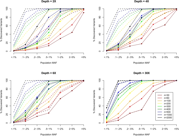
Figure 1 shows how the number of detected SNPs changes as a function of sequencing depth and the number of individuals sequenced by population MAF (i.e., MAF calculated using all 45,000 chromosomes). Rarer variants are more difficult to detect because it is challenging to distinguish genuine rare alleles from sequencing errors, particularly when individuals are sequenced at low depth. For example, suppose 100 individuals are sequenced, and two reads are obtained for every individual overlapping a particular locus. Further, suppose that two copies of the reference allele are observed in 99 of the sequenced individuals and that one copy of the reference allele and one copy of an alternative allele are observed in the 100th individual. With a sequencing error of ∼0.5% and no additional information, it would be impossible to tell if the alternative allele reflects a true heterozygote or a sequencing error. We see from Figure 1 that, whereas 100% of common variants with MAF > 5% can be detected when just 100 individuals are sequenced at depth 2×, only ∼3.8% of variants with MAF < 0.1% (<45 copies of the minor allele among the 45,000 chromosomes) can be detected even when 500 individuals are sequenced at depth 6×. The proportion of variants identified is bounded upwards by the proportion of polymorphisms in the population that segregate among sequenced individuals, which varies with MAF. For example, the chance that a MAF = 5% SNP is polymorphic among 60 individuals is ∼99.8%, while for a MAF = 0.1% SNP, it is only 11.3%. Dotted lines in Figure 1 show this theoretical upper bound. For comparison, we also present the detection power at depth 30× (bottom right panel), which largely overlaps with the theoretical upper bound as expected. Effectively, as more individuals are sequenced, a larger fraction of the variants actually present in the sample can be identified. This is because SNP discovery is dominated by two factors: the number of times the alternate allele is present among sequenced individuals, and the number of individuals where multiple reads support the alternate allele. Lastly, for low-frequency SNPs, the power of variant detection is also heavily influenced by the number of false positives allowed, which are tabulated in Supplemental Table 1. In general, we allowed more false positives when fewer individuals were sequenced.

Figure 1.

SNP discovery (%) by MAF, sequencing depth, and sequencing sample size. We simulated 30–2000 individuals sequenced at depths 2×, 4×, 6×, and 30×. We plotted the % of SNPs discovered by population MAF category (<0.1% to >5%), where population MAF is for the 45,000 simulated chromosomes. The dotted lines show the % of SNPs in each population MAF category that is polymorphic among the sequenced individuals.

Genotyping accuracy: Simulations

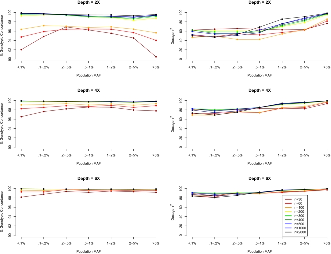
The proposed method estimates individual genotypes for detected variants. Figure 2 presents the genotypic concordance and r2 by minor allele frequency, with the former being the percentage of genotypes inferred correctly when genotypes assigned by the proposed model are compared with the true simulated genotypes, and the latter being the squared correlation between the inferred allele dosages (estimated fractional counts of an arbitrary allele for each SNP, ranging from 0.0 to 2.0) and the true allele counts (an integer quantity taking values 0, 1, or 2). While the first measure is a natural summary of genotyping accuracy, the latter measure is more directly related to power and sample size requirements for association mapping (Pritchard and Przeworski 2001).

Figure 2.

Genotype calling quality by MAF, sequencing depth, and sequencing sample size. We simulated 30–2000 individuals sequenced at depths 2×, 4×, and 6×. We compared genotype calls at detected SNPs with the simulated truth to obtain two measures of genotype calling quality, genotypic concordance and dosage r2, for each called SNP. We plot these two measures (left panel: genotypic concordance; right panel: dosage r2) by population MAF category (<0.1% to >5%), where population MAF is for the 45,000 simulated chromosomes.

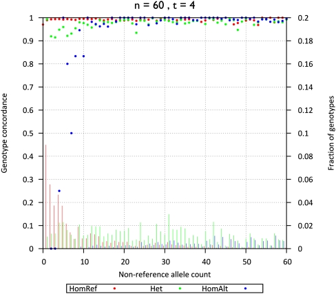
Figure 2 shows that highly accurate genotype inference can be made using lower depth sequencing. At depth 4×, >98% genotypic concordance is achieved across the examined MAF spectrum with as few as 60 sequenced individuals. For sites with low MAF, the overall genotypic concordance measure can be misleading because a rate of (1−MAF)2 × 100% can be achieved by simply assigning all individuals to be homozygous for the reference allele. (Such a strategy, while “accurate”, would not be helpful for genetic association studies. Comparisons with such a “straw-man” approach are presented in Supplemental Figure 1.) In general, rarer genotypes are more difficult to call, and this is reflected in lower concordance rates for heterozygotes and minor allele homozygotes (Fig. 3; Supplemental Figs. 2 and 3) as well as in lower values of the r2 statistic for markers with low MAF (Fig. 2, right panel). To improve accuracy for sites with a low minor allele frequency, it is necessary to increase sample size (see Supplemental Figs. 2 and 3). Note also that as sample size increases, the fraction of genotypes falling into the most difficult to call configurations (i.e., where the true genotypes are non-reference homozygotes at a low frequency variant site) decreases. For example, while ∼2% of genotypes are non-reference homozygotes for alleles with count <10 when 30 individuals are sequenced at 2× (Supplemental Fig. 2), <0.2% genotypes fall under that category when 500 individuals are sequenced at 6× (Supplemental Fig. 3).

Figure 3.

Genotype concordance and fraction of genotypes by non-ancestral allele counts (60 individuals sequenced at 4×). Genotype concordance (_y_-axis on left, dots) and fraction of genotypes (_y_-axis on right, bars) for simulated data, broken down by genotype category (homozygotes for the ancestral allele [HomRef], heterozygotes [Het], and homozygotes for the non-ancestral allele [HomAlt]) are plotted as a function of non-ancestral allele count among 60 individuals sequenced at 4× (_x_-axis).

Counter intuitively, dosage r2 for sites with low MAF can decrease with increasing sample size, for example, for SNPs with MAF 0.1%–0.2%, r2 is 64% when 30 individuals are sequenced at 2× but 53% when 500 individuals are sequenced at the same depth. We anticipated that the LD-based HMM, by borrowing information across individuals, would generate haplotypes that are progressively more accurate as additional individuals are sequenced. This is counterbalanced by a “winner's curse” phenomenon: Calling accuracy (measured by genotypic concordance or per-marker information content, n × r2) can only be evaluated at detected polymorphic sites, and larger samples, which allow detection of many more polymorphic sites, also include many configurations that are harder to call. When we repeated our evaluation but focused only on sites that were detected at all sequencing depths (which we call “easy-to-detect” sites), we found that dosage r2 increased with sample size as expected. For example, for a fixed set of detected SNPs with MAF < 0.5% and average sequencing depth of 2×, average r2 increased from 66% to 80% to 94% as sample size increased from 30 to 100 to 500 (Supplemental Fig. 4). As expected, the improved performance in larger samples is partly explained by the increasingly long stretches of chromosome shared among sequenced individuals, which become progressively easier for the LD-aware model to identify. These longer stretches likely originate in a more recent common ancestor and are also less likely to be disturbed by mutation or gene conversion events.

SNP discovery and genotype accuracy: Empirical evaluation

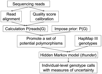
While analyses of simulated data can highlight important features of the proposed LD-aware method, they don't take into account many of the practical challenges of deploying low-coverage sequencing in real life settings. For example, in real data sets, many short reads might be mismapped, creating false evidence for polymorphisms. In addition, incorrect alignment of sequences near short insertion deletion polymorphisms might generate false evidence for SNPs and further disrupt calling. To evaluate the real life performance of the proposed methods, we used data generated by the 1000 Genomes Project (The 1000 Genomes Project Consortium 2010). The 1000 Genomes Project aims to detect all variants with frequency >1% in several continental regions by sequencing ∼2500 unrelated individuals at ∼4×depth. In its pilot phase, the project sequenced 179 unrelated individuals from the CEU, CHB+JPT, and YRI populations at an average depth of 2–4×. We used the proposed HMM model to analyze the data (using the steps summarized in Fig. 4). Since individuals sequenced in this low-coverage pilot were also genotyped at ∼1.4 million SNPs in Phase III of the International HapMap Project (The International HapMap Consortium 2007) using the Illumina 1M and the Affymetrix 6.0 SNP arrays, and we expected that a scaffold of high quality genotypes might aid the model's ability to identify shared haplotypes, we integrated these HapMap 3 genotypes into our analysis of the sequence data. Here, we also repeated our analysis removing HapMap genotype information so that results can be fairly compared with those from simulations. Since the number of individuals with genotypes at HapMap 2 specific sites varies among CEU, CHB+JPT, and YRI, our comparisons all use a random subset of 43 individuals for each panel (43 CEU, 43 CHB+JPT, and the 43 YRI) and for our simulated data.

Figure 4.

Genotype calling pipeline for the 1000 Genomes Pilot 1 Project. The pipeline we have developed to call genotypes for individuals sequenced at an average depth of ∼4–5× by the 1000 Genomes Pilot 1 Project.

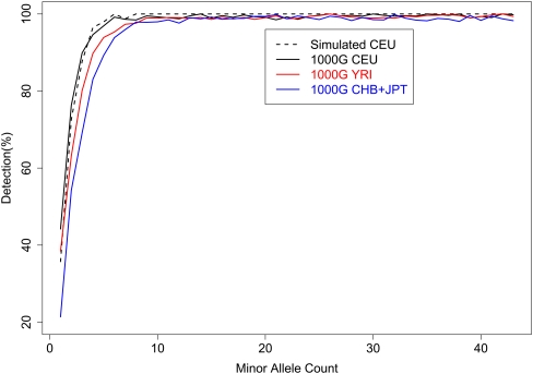
Figure 5 illustrates detection power by plotting the percentage of HapMap sites detected by minor allele count (out of 43). As expected, less common SNPs are harder to detect: Only 21%–44% of singleton SNPs and 54%–76% of doubleton SNPs can be detected, but 96%–100% of SNPs with a minor allele appearing 6–10 times were detected. We note that, by examining sequence data for 60 individuals but array genotypes for only 43 individuals, our results may overestimate detection power for a given minor allele count (particularly for singletons and doubletons) but underestimate detection power for a given minor allele frequency. For example, when 60 CEU samples are sequenced, nominal power to detect singletons is estimated to be 35.6%, 45.1%, and 65.3%, if the evaluation uses 60, 40, or 20 individuals, respectively (Supplemental Table 2). This finding can be easily explained: When assessing detection rate by minor allele count (MAC), some singleton SNPs (MAC = 1) among 20 or 40 individuals might correspond to alleles seen multiple times among the 60 sequenced individuals. For MAF = 2.5%, the detection rates are 65.3%, 81.7%, and 87.7%, respectively, when evaluation focuses on SNPs discovered among 20 individuals (MAC = 1), 40 individuals (MAC = 2), and among 60 individuals (MAC = 3). In this latter case, note that several of the SNPs seen once among 20 individuals may actually have frequency <2.5% in the larger set of 60 sequenced individuals.

Figure 5.

SNP detection power by minor allele count. For both simulated CEU and real data sets from the 1000 Genomes Project, SNPs were detected through a joint analysis of 59 or 60 individuals. Power of SNP detection was evaluated using a subset of 43 individuals.

For each called SNP, the model estimates r2 between called genotypes and (unobserved) true genotypes as a measure of genotype call accuracy. As expected, we have found that excluding sites with low estimated r2 results in higher quality sets of SNP calls (Browning and Yu 2009; Li et al. 2010b). For example, in the original calls for the 1000 Genomes CEU sample, focusing on sites with r2 greater than 0.0, 0.3, and 0.5 increases the ratio of transition to transversion SNPs from 1.86 to 1.88 and then to 1.97, excluding 0%, 5%, and 17% of the initial set of SNPs. For known sites, this ratio slightly exceeds 2.0 across the genome and is often used to evaluate overall SNP call set quality (Zhao and Boerwinkle 2002; Zhang and Gerstein 2003).

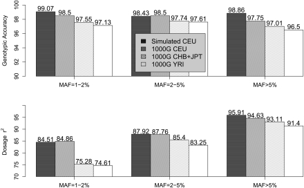
Genotype calling accuracy in the 1000 Genomes Project Pilot samples (CEU, CHB+JPT, and YRI), measured by overall genotypic concordance and dosage r2, is presented in Figure 6, together with a summary of performance in our previously described simulations. Reassuringly, analysis of simulated and real data led to similar SNP discovery rates and genotype accuracies (measured either as the fraction of concordant genotypes or using the dosage r2 measure). For example, empirical genotypic concordance among the CEU samples is >98%, very close to expectations from simulations. While genotypic concordance varies little with MAF, in the range examined the more informative r2 measure increases with MAF, from ∼85% for SNPs with MAF 1%–2%, to 88% for MAF 2%–5%, and to ∼95% for MAF > 5%. Performance among the CHB+JPT and YRI samples was slightly worse, particularly for rarer SNPs, likely due to somewhat lower depth of coverage in these two sample sets (The 1000 Genomes Project Consortium 2010) and to the lower level of LD in YRI. In addition, we present in Supplemental Figure 5 results when phase 3 HapMap genotypes were integrated into analysis. As expected, calling accuracy improved with the additional genotype data but not substantially. For example, r2 increased from 84.86%, 75.28%, and 74.61% to 85.78%, 76.77%, and 76.18%, respectively, for CEU, CHB+JPT, and YRI for SNPs with MAF 1%–2%.

Figure 6.

Genotype calling quality: Simulated versus the 1000 Genomes Pilot 1. Genotype calling quality is gauged by two measures—genotypic concordance and dosage r2—by comparing with true genotypes in simulated data and with experimental genotypes in real data from the 1000 Genomes Low-coverage Pilot Project. For both the real and simulated data, 60 individuals were sequenced at an average depth of 4×. For the 1000 Genomes Pilot 1 data, genotype calling was performed using sequencing data alone without HapMap 3 genotypes.

Low-coverage versus high-coverage sequencing designs

We have so far shown that low-coverage sequencing of many individuals can be used to detect polymorphic sites and infer genotypes when many individuals are sequenced, each at 2×–6× depth. This capability has important implications for the design of complex disease association studies, which require large sample sizes to detect genetic variants of modest effect. The typical GWAS examines several thousand individuals (McCarthy et al. 2008), and, for a number of diseases/traits, meta-analyses involving >100,000 individuals have been carried out (Lindgren et al. 2009; Newton-Cheh et al. 2009; Dupuis et al. 2010; Teslovich et al. 2010). We expect that affordable designs for sequencing large numbers of samples will be critically important for the successful transition from GWAS to sequencing-based association studies. Given that total sequencing capacity is limited, low-coverage sequencing allows much larger numbers of individuals to be studied.

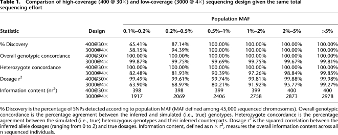
We first simulated two extreme alternatives using the same procedure described earlier. The first included sequence data for 400 individuals, each covered at 30× average read depth. The second included sequence data for 3000 individuals, each covered at 4× average read depth. Both designs result in the same total investment of sequencing capacity. Table 1 summarizes five statistics for the two designs: (1) the percentage of detected sites, (2) the overall genotype concordance, (3) heterozygote concordance (which is a more challenging benchmark of genotyping accuracy), (4) dosage r2, and (5) total information content as measured by _n_r2, where n is the number of individuals sequenced. Both designs had nearly 100% power to detect variants with MAF > 0.5%, while the low-coverage design provided greater power to detect less common variants with MAF 0.2%–0.5%. Neither design had much power for the rarest SNPs (MAF < 0.1%). For high-coverage designs, the minor allele for rare SNPs was often absent from the sequenced sample; for low-coverage designs, it was not possible to distinguish true variants from sequencing errors confidently with a small number of non-reference reads.

Table 1.

Comparison of high-coverage (400 @ 30×) and low-coverage (3000 @ 4×) sequencing design given the same total sequencing effort

For detected variants, genotype accuracy was reduced for low-coverage designs compared to high-coverage designs but was still impressive. For example, for variants with MAF > 1%, the genotypic concordance was always >99.67%, and concordance at heterozygous sites was >97%. As noted previously, high rates of polymorphism discovery and reasonably accurate genotype inference are possible because the model effectively combines information across individuals with similar haplotypes, so that the coverage of each haplotype is, effectively, quite deep. Thus, low-coverage designs substantially increase the overall information content (even when genotypes are individually not as good, in aggregate, they contain more information), holding the overall sequencing investment constant. For example, for variants with MAF 0.1%–0.2%, 0.2%–0.5%, 0.5%–1.0%, 1.0%–2.0%, or 2.0%–5.0%, 4× sequencing of 3000 individuals provided effective sample sizes measured by _n_r2 of 1917, 2069, 2406, 2758, and 2873, corresponding to an effective sample size 4.8×, 5.2×, 6.0×, 6.9×, and 7.2× greater than if 30× sequencing of 400 individuals were carried out. Note that the boost in effective sample size holds for any disease allele effect size.

Power of several design options for sequencing-based genetic association studies

To quantify further the benefits of low-coverage designs for association mapping, we carried out simulation studies directly assessing statistical power to detect disease-SNP association. For each of the ten regions, we simulated 50 replicates of 1500 cases and 1500 controls, assuming one causal SNP per simulated replicate per region. We focused on scenarios where the causal variant is a low-frequency SNP with MAF ∼0.1%, ∼0.5%, ∼1%, or ∼3%. For each disease MAF, the effect size [as measured by genetic relative risk (GRR)] was selected using CaTS (Skol et al. 2006) to achieve ∼60% power when the causal SNP was genotyped in 1000 cases and 1000 controls and tested for association at a significance threshold of 0.05/200 = 0.00025 (200 is the approximate number of independent tests in each sequenced region). This resulted in a GRR of 8.27, 3.25, 2.45, and 1.77 respectively, for 0.1%, 0.5%, 1%, and 3% disease MAF, respectively. In parallel, we simulated 50 null sets by randomly sampling 6000 chromosomes from the pool of 45,000 chromosomes and assigning these to the 1500 cases and 1500 controls at random.

We compared the following designs: tagSNP genotyping of all 3000 samples, sequencing all 3000 individuals at depth 4×, sequencing progressively smaller numbers of individuals (2000, 1000, and 400) at progressively higher depths (6×, 12×, 30×), and a final set of designs that augment available sequence data through imputation of discovered alleles into the remaining individuals, using the tagSNP genotypes as a scaffold. TagSNPs were picked to mimic Illumina HumanHap650K with an average coverage of 88% of the common (MAF > 5%) SNPs (see Li et al. 2010b for details). We used our packages MaCH and Thunder to generate genotype calls, estimate allele dosages for sequenced individuals, and impute genotypes from sequenced individuals into the remaining individuals. Association analysis was performed using logistic regression with allele dosages as the explanatory variable. Significance thresholds were calibrated using the 500 null replicates and selected to achieve a family-wise error rate of 5%.

Power is summarized in Table 2. First, consistent with the substantial increase in information content shown in Table 1, power increases substantially when sample size increases from 400 to 3000: from 4.0% to 61.6%, 6.4% to 75.6%, 7.4% to 82.8%, and 11.6% to 90.4% when disease MAF is 0.1%, 0.5%, 1%, or 3%, respectively. In general, with fixed sequencing effort (total 12,000× for the four different sequencing designs evaluated), low-coverage sequencing of more individuals increases power compared to high-coverage sequencing of fewer individuals.

Table 2.

Comparison of power to detect disease-SNP association: tagSNPs only; different sequencing designs with fixed sequencing cost; and different sequencing designs with fixed sequencing cost plus imputation in additional individuals not sequenced

Second, when a relatively small number of individuals are sequenced, power can actually be lower than for designs that use tagSNPs alone but examine larger numbers of individuals. For example, in our simulation, tagSNP genotyping of 3000 individuals had 30.8% power to detect disease-associated loci with MAF of ∼3%, but sequencing of 400 individuals at 30× depth had only 11.6% power for the same MAF. This observation implies that deep sequencing of modest numbers of individuals, although it allows direct examination of much larger numbers of variants, may not necessarily lead to new disease susceptibility loci that were missed in GWAS.

Third, imputation from sequenced individuals into additional genotyped individuals can be extremely efficient. For example, power increases from 17.8% to 41.8% for a 3% disease MAF when variants detected in 1000 individuals sequenced at 12× are imputed into the remaining 2000 individuals.

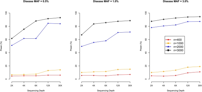
Fourth, we evaluated 20 combinations of sample size and sequencing depth (sample size taking values 400, 1000, 2000, and 3000 and sequencing depth taking values 2, 4, 6, 12, and 30, including the two designs assessed in Table 1) and directly assessed power to detect disease SNPs with MAF 0.5%, 1%, or 3% (Fig. 7). As expected, for the same number of individuals sequenced, power increases with sequencing depth. For example, power increases by an average of 8% when depth increases from 4× to 12× (i.e., tripling sequencing effort). However, power typically increases even more when total sequencing effort is increased by increasing the number of sequenced individuals. For example, power is 7% for disease MAF 0.5% when sequencing 1000 individuals at 4×. If we increase total sequencing effort to 12,000×, we can (1) sequence the same 1000 individuals, increasing coverage to 12×, or (2) sequence a total of 3000 individuals at 4×. Option 1 results in 13.4% power (6.4% power gain), while Option 2 results in 75.6% power (68.6% power gain).

Figure 7.

Power of association mapping by sequencing depth and number of individuals sequenced. We simulated 1500 cases and 1500 controls, assuming a single causal variant with causal allele frequency 0.5%, 1%, or 3%. We sequenced all 3000 individuals or a random subset of 400, 1000, or 2000 individuals (equal number of cases and controls) at depths ranging from 2×–30×. Power was estimated using an empirical threshold determined from 500 null sets to ensure familywise type-I error of 5%.

Reference panels based on low-coverage sequencing

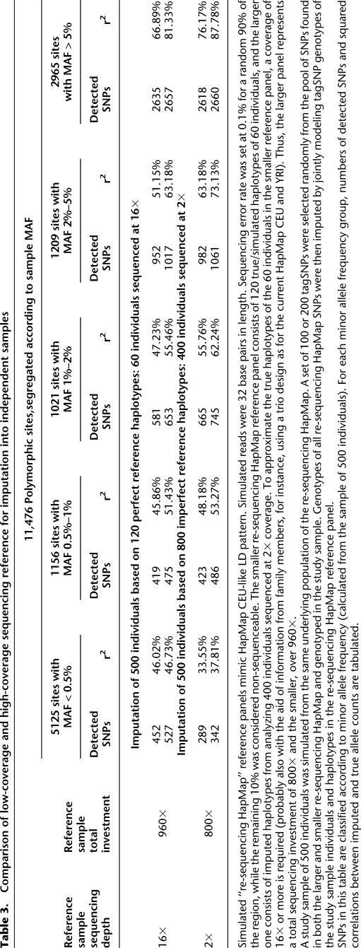
Eventually, we expect that low-coverage sequencing will be deployed in the context of many genetic association studies. In the interim, many investigators will consider using the haplotypes derived by low coverage sequencing of the 1000 Genomes Project samples (or other samples) to impute missing genotypes in their own samples. Thus, we set out to evaluate whether haplotypes estimated using low-pass sequencing could provide a good reference for imputation of cataloged variants into existing GWAS data. Table 3 compares the utility of two alternative extreme designs for building such a reference. In one design, 60 individuals are sequenced deeply at 16×. In the alternative design, 400 individuals are sequenced at 2×. Roughly, these correspond to two hypothetical designs considered at the outset of the 1000 Genomes Project (The 1000 Genomes Project Consortium 2010). In each case, we evaluate the utility of the resulting panel for imputation into additional samples typed only for GWAS tagSNPs. For SNPs with MAF > 0.5%, the low-coverage design clearly manifests its advantages in terms of both variant discovery power and information content after imputation. For example, 14% more SNPs with MAF 1%–2% can be imputed (with r2 > 0.3) using the haplotypes derived from low-coverage sequencing of 400 individuals than using haplotypes derived from deeper sequencing of 60 individuals. For SNPs that can be imputed, there is a ∼7% increase in r2 (from 55.46% to 62.24%) when imputed and true simulated genotypes are compared in individuals typed at tag SNPs only. We, therefore, believe that low-coverage sequencing is a practical strategy for building imputation reference panels.

Table 3.

Comparison of low-coverage and high-coverage sequencing reference for imputation into independent samples

Discussion

We have proposed and implemented an LD-based method for SNP discovery and genotype calling that combines sequence data across many individuals. Our method, by jointly analyzing all sequenced individuals and borrowing information from individuals carrying similar haplotypes, enables accurate genotype inference from low-coverage sequencing data. We have shown through simulation studies and analyses of data generated by the 1000 Genomes Pilot Project (The 1000 Genomes Project Consortium 2010) that when >50 individuals are sequenced, >98% genotypic concordance rate can be achieved for SNPs with >10 copies of the minor allele among individuals sequenced at depth ≥ 4×. Our simulations predict that, for a fixed sequencing depth, accuracy will improve further as additional individuals are sequenced, a prediction that early analyses of expanded 1000 Genomes Project data sets confirm. For example, when the number of individuals of European ancestry analyzed increased from 60 to 563, we were able to detect 105% more SNPs, and the overall genotype mismatch rate dropped from 1.61% to 0.59%.

One practical issue that we have not discussed concerns the rapid improvement of sequencing technologies, in terms of both increased read length and decreased sequencing error rates. Drops in sequencing error make both SNP detection and genotype calling more accurate. Similarly, longer read lengths, which reduce the proportion of mismapped reads, should also improve overall genotype accuracy. For example, simulations suggested that, as sequencing error rates drop from 1.0% to 0.5% to 0.1% and ultimately to 0%, the proportion of population SNPs with MAF 1%–2% that can be discovered through low-coverage sequencing of 100 individuals at depth 2× increases from 6.7% to12.4% to 23.1% and ultimately to 60.2%.

In the 1000 Genomes Project, genotypes were called using three independently developed methods for the analysis of low-coverage sequence data. In addition to the methodology described here, genotypes were initially called at the Sanger Center with QCALL (Le and Durbin 2010) and at the Broad with GATK (McKenna et al. 2010) and BEAGLE (Browning and Yu 2009). The methods differ from ours in several ways. For example, QCALL uses pre-existing genotype data to group individuals into “clades,” using an approximation to the local ancestral recombination graph of each region and then uses these groupings when making each genotype call. GATK and BEAGLE use variable length Markov chains to describe the LD structure in each region, a method that might be more robust to false SNPs than the approach used here. Interestingly, evaluation of the three methods in the 1000 Genomes Project data showed that, while they each have similar accuracy (Supplemental Table 3), combining results of the three methods into an integrated call set (using a majority vote rule) greatly improves genotype calling accuracy. For example, consensus genotypes for individuals of European ancestry (by comparing both the sites detected as SNPs and actual genotypes called) generated by merging calls from the three independent sets (available from the project ftp site at ftp://ftp-trace.ncbi.nih.gov/1000genomes/ftp/release/2010_11/) have average genotypic accuracy of 98.69% (compared to 97.56%–98.01% in any single call set). This observation suggests that there is still much room for refinement of individual genotype callers for low-coverage sequence data.

The possibility of deploying low-coverage sequencing to large sets of phenotyped samples has important implications for genetic association studies. While more research is needed to identify optimal designs, taking into account fixed per sample preparation costs, sequencing costs, and genotyping costs, the results presented here already offer two lessons. First, we have demonstrated that low-coverage designs are more powerful than deep sequencing of fewer individuals for medical sequencing studies when a large sample size is required for the detection of modest effect sizes or low-frequency causal variants, particularly by comparing the overall information content and statistical power of sequencing designs with the same total sequencing effort. Specifically, we find that it is generally preferable to sequence more individuals at low coverage than to sequence a smaller subset of individuals at deeper coverage. As the most recent wave of GWAS has collected more samples than can be practically sequenced (for now), low-coverage sequencing should provide an attractive means of using these large existing sample sets for the next round of complex trait studies. Second, imputation of variants detected through sequencing into the remainder of the sample further increases power for association mapping.

For sequencing-based association studies of complex traits, the trade-off between number of individuals sequenced and sequencing depth has important implications. For example, the only way to comprehensively detect singletons and other very rare variants remains to use deep sequencing and, if the focus is on such variants, there is no current practical alternative to deep sequencing of samples at depth 20×–30×. However, for common and low-frequency SNPs with MAF > 0.2%, we have demonstrated that the proposed LD-based hidden Markov model can make reasonably accurate inference when a large number of individuals is sequenced. Since the relative contributions of common, low-frequency, and very rare variants to complex trait variation remain unknown, the optimal design has not yet been identified.

Recent complex trait GWAS have presented the sobering fact that large sample sizes are key for studies of the genetic architecture of complex traits. We anticipate the proposed methods for analysis of low-coverage sequencing data will facilitate applications of the emerging sequencing technologies to the study of complex traits in very large numbers of individuals. While we have assessed the impact of the proposed methods using single variant tests, imputation-based analysis can be combined with aggregate tests for rare variants (Li et al. 2010a; Zawistowski et al. 2010).

Methods

We have developed LD-based methods for SNP detection and genotyping from massively parallel sequencing data, as an extension of our genotype-based imputation methods (Li et al. 2009c). Methods used for simulated data were previously outlined in Li et al. (2010b), based on a simple model that focused on the number of reads containing one of two alternate alleles at each position and in each individual. More generally, our method uses a series of likelihoods lk(reads|G) as input. Each of these gives the likelihood of observed read data when genotype G is assumed at location m. For each location, 10 possible genotypes (A/A, A/C, A/T, A/G, C/C, C/G, C/T, G/G, G/T, T/T) must be considered—allowing for single base deletions would result in an additional set of possible genotypes. These likelihoods can be calculated using a variety of models for short read sequence data. Here, we use the maq error model (Li et al. 2008), as implemented in SAMtools (Li et al. 2009a). The model considers the base calls and associated quality scores in each read, together with mapping quality and a simple model for artifacts due to small insertion and deletion polymorphisms. SAMtools can use short read alignments stored in SAM/BAM files to generate this information and store the results in Genotype Likelihood Format (GLF) files [see http://samtools.sourceforge.net/SAM1.pdf].

Starting with the genotype likelihoods stored in GLF files, we first select a set of sites that are more likely to be polymorphic based on a simple single site analysis. We then consider these sites jointly within a hidden Markov model where haplotypes are reconstructed by leveraging relatively short chromosome stretches shared across individuals. A typical workflow is depicted in Figure 4, and further details are provided in the remainder of this section.

Identification of potential polymorphic sites

The goal of this step is to focus more time-consuming analyses on likely polymorphic sites. Input data are likelihoods for each individual at each sequenced base pair lk(reads|G), where G takes the ten possible values {A/A, A/C, A/G, A/T, C/C, C/G, C/T, G/G, G/T, T/T}; subscripts indicating base pair and individual are suppressed for simplicity.

Since we only consider bi-allelic SNPs, we want to infer the following posterior probability for each sequenced base pair:

We impose the following prior based on population genetics principles (Hudson 1991):

Here, θ is the per base pair heterozygosity, typically on the order of 10−3 for humans. We further break down the polymorphism prior probabilities according to mutation type defined by the alleles in the reference genome:

where transitions refer to purine to purine (A↔G) or primidine to primidine (C↔T) mutations, while transversions refer to purine to primidine mutations (A or G↔C or T).

To infer the desired posterior probabilities, we need the likelihood which is proportional to the probability of the sequence data. We define the likelihood as a function of pa, the frequency of allele a:

where

Finally, we calculate the posterior as:

Sites that exceed a prespecified posterior probability cutoff are promoted as the set of likely polymorphic sites worthy of further analysis. For data from the 1000 Genomes Low-coverage Pilot we used 0.9 as the posterior probability cutoff.

Hidden Markov model

Our genotype calling method uses LD information and is based on the rationale that apparently unrelated individuals often share short stretches of chromosome. We use a hidden Markov model where the hidden state at each marker contains a pair of indices for the most closely related reference haplotypes for the stretch of chromosome being considered in each individual (Li et al. 2010b; Li et al. 2009c ). The observed data are the genotype likelihoods reported by SAMtools (Li et al. 2009a).

In sequencing-based studies, there is typically no external reference panel. Instead, interim haplotypes estimated for other sequenced individuals will be used as the reference. Given n sequenced diploid individuals, hidden state (x,y) can take [2(n - 1)]2 different values with x, _y_∈ {1,2,…, 2(n - 1)}.

Define Pr(Sm | reads) as the posterior probability for Sm, the hidden state at marker m with reads denoting the available sequencing data across all sites = (_reads_1, _reads_2, …, _reads_M), where M is the total number of polymorphisms considered. To calculate the posterior probabilities, we adopt Baum's forward and backward algorithm (Baum 1972). We calculate the forward probability:

and the backward probability:

To calculate the forward probabilities, we note that the emission probability at marker m:

In the standard formulation, forward probabilities are joint probabilities and backward are conditional such that the desired posterior probability:

For the rightmost marker M, Pr(SM = (x, y) | reads) ∝ Pr(reads, SM = (x, y)) ≡ fM(x, y).

With the posterior probabilities calculated, genotype calls can be conveniently inferred. For each individual at each locus, our method generates three measures of underlying genotype: (1) the most likely genotype: the genotype with the largest posterior probability; (2) genotype dosage: the estimated number of copies of an arbitrary reference allele; and (3) the posterior probabilities of the three possible genotypes. Each of these quantities is inferred by integrating over all possible hidden state configurations.

Acknowledgments

We thank Serena Sanna for helpful discussions. This research was supported by research grants from the NIMH, NHLBI, and the NHGRI to G.R.A. and HG000376 to M.B. Y.L. is partially supported by NIH grant 3-R01-CA082659-11S1.

Footnotes

References

1. The 1000 Genomes Project Consortium 2010. A map of human genome variation from population-scale sequencing. Nature 467: 1061–1073 [DOI] [PMC free article] [PubMed] [Google Scholar]
2. Bansal V, Harismendy O, Tewhey R, Murray SS, Schork NJ, Topol EJ, Frazer KA 2010. Accurate detection and genotyping of SNPs utilizing population sequencing data. Genome Res 20: 537–545 [DOI] [PMC free article] [PubMed] [Google Scholar]
3. Baum LE 1972. An inequality and associated maximization technique in statistical estimation for probabilistic functions of Markov processes. Inequalities 3: 1–8 [Google Scholar]
4. Bentley DR 2006. Whole-genome re-sequencing. Curr Opin Genet Dev 16: 545–552 [DOI] [PubMed] [Google Scholar]
5. Bentley DR, Balasubramanian S, Swerdlow HP, Smith GP, Milton J, Brown CG, Hall KP, Evers DJ, Barnes CL, Bignell HR, et al. 2008. Accurate whole human genome sequencing using reversible terminator chemistry. Nature 456: 53–59 [DOI] [PMC free article] [PubMed] [Google Scholar]
6. Browning BL, Yu Z 2009. Simultaneous genotype calling and haplotype phasing improves genotype accuracy and reduces false-positive associations for genome-wide association studies. Am J Hum Genet 85: 847–861 [DOI] [PMC free article] [PubMed] [Google Scholar]
7. Dupuis J, Langenberg C, Prokopenko I, Saxena R, Soranzo N, Jackson AU, Wheeler E, Glazer NL, Bouatia-Naji N, Gloyn AL, et al. 2010. New genetic loci implicated in fasting glucose homeostasis and their impact on type 2 diabetes risk. Nat Genet 42: 105–116 [DOI] [PMC free article] [PubMed] [Google Scholar]
8. Hindorff LA, Sethupathy P, Junkins HA, Ramos EM, Mehta JP, Collins FS, Manolio TA 2009. Potential etiologic and functional implications of genome-wide association loci for human diseases and traits. Proc Natl Acad Sci 106: 9362–9367 [DOI] [PMC free article] [PubMed] [Google Scholar]
9. Hudson RR 1991. Gene genealogies and the coalescent process. In Oxford Surveys in Evolutionary Biology, Vol. 7 (ed. D Futuyma, J Antonovics), pp. 1–44. Oxford University Press, New York. [Google Scholar]
10. The International HapMap Consortium 2007. A second generation human haplotype map of over 3.1 million SNPs. Nature 449: 851–861 [DOI] [PMC free article] [PubMed] [Google Scholar]
11. Le SQ, Durbin R 2011. SNP detection and genotyping from low-coverage sequencing data on multiple diploid samples. Genome Res (this issue). doi: 10.1101/gr.113084.110 [DOI] [PMC free article] [PubMed] [Google Scholar]
12. Ley TJ, Mardis ER, Ding L, Fulton B, McLellan MD, Chen K, Dooling D, Dunford-Shore BH, McGrath S, Hickenbotham M, et al. 2008. DNA sequencing of a cytogenetically normal acute myeloid leukaemia genome. Nature 456: 66–72 [DOI] [PMC free article] [PubMed] [Google Scholar]
13. Li H, Ruan J, Durbin R 2008. Mapping short DNA sequencing reads and calling variants using mapping quality scores. Genome Res 18: 1851–1858 [DOI] [PMC free article] [PubMed] [Google Scholar]
14. Li H, Handsaker B, Wysoker A, Fennell T, Ruan J, Homer N, Marth G, Abecasis G, Durbin R 2009a. The Sequence Alignment/Map format and SAMtools. Bioinformatics 25: 2078–2079 [DOI] [PMC free article] [PubMed] [Google Scholar]
15. Li RQ, Li YR, Fang XD, Yang HM, Wang J, Kristiansen K 2009b. SNP detection for massively parallel whole-genome resequencing. Genome Res 19: 1124–1132 [DOI] [PMC free article] [PubMed] [Google Scholar]
16. Li Y, Willer C, Sanna S, Abecasis G 2009c. Genotype imputation. Annu Rev Genomics Hum Genet 10: 387–406 [DOI] [PMC free article] [PubMed] [Google Scholar]
17. Li Y, Byrnes AE, Li M 2010a. To identify associations with rare variants, just WHaIT: Weighted Haplotype and Imputation-Based Tests. Am J Hum Genet 87: 728–735 [DOI] [PMC free article] [PubMed] [Google Scholar]
18. Li Y, Willer CJ, Ding J, Scheet P, Abecasis GR 2010b. MaCH: Using sequence and genotype data to estimate haplotypes and unobserved genotypes. Genet Epidemiol 34: 816–834 [DOI] [PMC free article] [PubMed] [Google Scholar]
19. Lindgren CM, Heid IM, Randall JC, Lamina C, Steinthorsdottir V, Qi L, Speliotes EK, Thorleifsson G, Willer CJ, Herrera BM, et al. 2009. Genome-wide association scan meta-analysis identifies three loci influencing adiposity and fat distribution. PLoS Genet 5: doi: 10.1371/journal.pgen.1000508 [DOI] [PMC free article] [PubMed] [Google Scholar]
20. Lupski JR, Reid JG, Gonzaga-Jauregui C, Rio Deiros D, Chen DC, Nazareth L, Bainbridge M, Dinh H, Jing C, Wheeler DA, et al. 2010. Whole-genome sequencing in a patient with Charcot-Marie-Tooth neuropathy. N Engl J Med 362: 1181–1191 [DOI] [PMC free article] [PubMed] [Google Scholar]
21. Maher B 2008. Personal genomes: The case of the missing heritability. Nature 456: 18–21 [DOI] [PubMed] [Google Scholar]
22. Manolio TA, Collins FS, Cox NJ, Goldstein DB, Hindorff LA, Hunter DJ, McCarthy MI, Ramos EM, Cardon LR, Chakravarti A, et al. 2009. Finding the missing heritability of complex diseases. Nature 461: 747–753 [DOI] [PMC free article] [PubMed] [Google Scholar]
23. Mardis ER 2008. Next-generation DNA sequencing methods. Annu Rev Genomics Hum Genet 9: 387–402 [DOI] [PubMed] [Google Scholar]
24. Margulies M, Egholm M, Altman WE, Attiya S, Bader JS, Bemben LA, Berka J, Braverman MS, Chen YJ, Chen Z, et al. 2005. Genome sequencing in microfabricated high-density picolitre reactors. Nature 437: 376–380 [DOI] [PMC free article] [PubMed] [Google Scholar]
25. McCarthy MI, Abecasis GR, Cardon LR, Goldstein DB, Little J, Ioannidis JP, Hirschhorn JN 2008. Genome-wide association studies for complex traits: Consensus, uncertainty, and challenges. Nat Rev Genet 9: 356–369 [DOI] [PubMed] [Google Scholar]
26. McKenna A, Hanna M, Banks E, Sivachenko A, Cibulskis K, Kernytsky A, Garimella K, Altshuler D, Gabriel S, Daly M, et al. 2010. The Genome Analysis Toolkit: a MapReduce framework for analyzing next-generation DNA sequencing data. Genome Res 20: 1297–1303 [DOI] [PMC free article] [PubMed] [Google Scholar]
27. Newton-Cheh C, Johnson T, Gateva V, Tobin MD, Bochud M, Coin L, Najjar SS, Zhao JH, Heath SC, Eyheramendy S, et al. 2009. Genome-wide association study identifies eight loci associated with blood pressure. Nat Genet 41: 666–676 [DOI] [PMC free article] [PubMed] [Google Scholar]
28. Ng SB, Turner EH, Robertson PD, Flygare SD, Bigham AW, Lee C, Shaffer T, Wong M, Bhattacharjee A, Eichler EE, et al. 2009. Targeted capture and massively parallel sequencing of 12 human exomes. Nature 461: 272–276 [DOI] [PMC free article] [PubMed] [Google Scholar]
29. Ng SB, Buckingham KJ, Lee C, Bigham AW, Tabor HK, Dent KM, Huff CD, Shannon PT, Jabs EW, Nickerson DA, et al. 2010. Exome sequencing identifies the cause of a Mendelian disorder. Nat Genet 42: 30–35 [DOI] [PMC free article] [PubMed] [Google Scholar]
30. Nikopoulos K, Gilissen C, Hoischen A, van Nouhuys CE, Boonstra FN, Blokland EAW, Arts P, Wieskamp N, Strom TM, Ayuso C, et al. 2010. Next-generation sequencing of a 40 Mb linkage interval reveals TSPAN12 mutations in patients with familial exudative vitreoretinopathy. Am J Hum Genet 86: 240–247 [DOI] [PMC free article] [PubMed] [Google Scholar]
31. Pritchard JK, Przeworski M 2001. Linkage disequilibrium in humans: Models and data. Am J Hum Genet 69: 1–14 [DOI] [PMC free article] [PubMed] [Google Scholar]
32. Roach JC, Glusman G, Smit AF, Huff CD, Hubley R, Shannon PT, Rowen L, Pant KP, Goodman N, Bamshad M, et al. 2010. Analysis of genetic inheritance in a family quartet by whole-genome sequencing. Science 328: 636–639 [DOI] [PMC free article] [PubMed] [Google Scholar]
33. Schaffner SF, Foo C, Gabriel S, Reich D, Daly MJ, Altshuler D 2005. Calibrating a coalescent simulation of human genome sequence variation. Genome Res 15: 1576–1583 [DOI] [PMC free article] [PubMed] [Google Scholar]
34. Shendure J, Ji HL 2008. Next-generation DNA sequencing. Nat Biotechnol 26: 1135–1145 [DOI] [PubMed] [Google Scholar]
35. Skol AD, Scott LJ, Abecasis GR, Boehnke M 2006. Joint analysis is more efficient than replication-based analysis for two-stage genome-wide association studies. Nat Genet 38: 209–213 [DOI] [PubMed] [Google Scholar]
36. Teslovich TM, Musunuru K, Smith AV, Edmondson AC, Stylianou IM, Koseki M, Pirruccello JP, Ripatti S, Chasman DI, Willer CJ, et al. 2010. Biological, clinical, and population relevance of 95 loci for blood lipids. Nature 466: 707–713 [DOI] [PMC free article] [PubMed] [Google Scholar]
37. Willer CJ, Li Y, Abecasis GR 2010. METAL: Fast and efficient meta-analysis of genomewide association scans. Bioinformatics 26: 2190–2191 [DOI] [PMC free article] [PubMed] [Google Scholar]
38. Zawistowski M, Gopalakrishnan S, Ding J, Li Y, Grimm S, Zollner S 2010. Extending rare-variant testing strategies: Analysis of noncoding sequence and imputed genotypes. Am J Hum Genet 87: 604–617 [DOI] [PMC free article] [PubMed] [Google Scholar]
39. Zhang ZL, Gerstein M 2003. Patterns of nucleotide substitution, insertion and deletion in the human genome inferred from pseudogenes. Nucleic Acids Res 31: 5338–5348 [DOI] [PMC free article] [PubMed] [Google Scholar]
40. Zhao Z, Boerwinkle E 2002. Neighboring-nucleotide effects on single nucleotide polymorphisms: A study of 2.6 million polymorphisms across the human genome. Genome Res 12: 1679–1686 [DOI] [PMC free article] [PubMed] [Google Scholar]