make_lsq_spline — SciPy v1.15.2 Manual (original) (raw)

scipy.interpolate.

scipy.interpolate.make_lsq_spline(x, y, t, k=3, w=None, axis=0, check_finite=True, *, method='qr')[source]#

Compute the (coefficients of) an LSQ (Least SQuared) based fitting B-spline.

The result is a linear combination

\[S(x) = \sum_j c_j B_j(x; t)\]

of the B-spline basis elements, \(B_j(x; t)\), which minimizes

\[\sum_{j} \left( w_j \times (S(x_j) - y_j) \right)^2\]

Parameters:

xarray_like, shape (m,)

Abscissas.

yarray_like, shape (m, …)

Ordinates.

tarray_like, shape (n + k + 1,).

Knots. Knots and data points must satisfy Schoenberg-Whitney conditions.

kint, optional

B-spline degree. Default is cubic, k = 3.

warray_like, shape (m,), optional

Weights for spline fitting. Must be positive. If None, then weights are all equal. Default is None.

axisint, optional

Interpolation axis. Default is zero.

check_finitebool, optional

Whether to check that the input arrays contain only finite numbers. Disabling may give a performance gain, but may result in problems (crashes, non-termination) if the inputs do contain infinities or NaNs. Default is True.

methodstr, optional

Method for solving the linear LSQ problem. Allowed values are “norm-eq” (Explicitly construct and solve the normal system of equations), and “qr” (Use the QR factorization of the design matrix). Default is “qr”.

Returns:

ba BSpline object of the degree k with knots t.

Notes

The number of data points must be larger than the spline degree k.

Knots t must satisfy the Schoenberg-Whitney conditions, i.e., there must be a subset of data points x[j] such thatt[j] < x[j] < t[j+k+1], for j=0, 1,...,n-k-2.

Examples

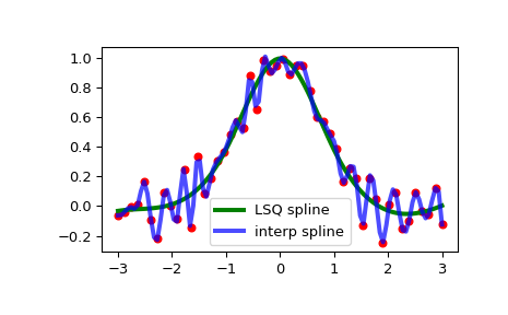
Generate some noisy data:

import numpy as np import matplotlib.pyplot as plt rng = np.random.default_rng() x = np.linspace(-3, 3, 50) y = np.exp(-x**2) + 0.1 * rng.standard_normal(50)

Now fit a smoothing cubic spline with a pre-defined internal knots. Here we make the knot vector (k+1)-regular by adding boundary knots:

from scipy.interpolate import make_lsq_spline, BSpline t = [-1, 0, 1] k = 3 t = np.r_[(x[0],)(k+1), ... t, ... (x[-1],)(k+1)] spl = make_lsq_spline(x, y, t, k)

For comparison, we also construct an interpolating spline for the same set of data:

from scipy.interpolate import make_interp_spline spl_i = make_interp_spline(x, y)

Plot both:

xs = np.linspace(-3, 3, 100) plt.plot(x, y, 'ro', ms=5) plt.plot(xs, spl(xs), 'g-', lw=3, label='LSQ spline') plt.plot(xs, spl_i(xs), 'b-', lw=3, alpha=0.7, label='interp spline') plt.legend(loc='best') plt.show()

NaN handling: If the input arrays contain nan values, the result is not useful since the underlying spline fitting routines cannot deal withnan. A workaround is to use zero weights for not-a-number data points:

y[8] = np.nan w = np.isnan(y) y[w] = 0. tck = make_lsq_spline(x, y, t, w=~w)

Notice the need to replace a nan by a numerical value (precise value does not matter as long as the corresponding weight is zero.)