csd — SciPy v1.16.2 Manual (original) (raw)
scipy.signal.
scipy.signal.csd(x, y, fs=1.0, window='hann', nperseg=None, noverlap=None, nfft=None, detrend='constant', return_onesided=True, scaling='density', axis=-1, average='mean')[source]#
Estimate the cross power spectral density, Pxy, using Welch’s method.
Parameters:
xarray_like
Time series of measurement values
yarray_like
Time series of measurement values
fsfloat, optional
Sampling frequency of the x and y time series. Defaults to 1.0.
windowstr or tuple or array_like, optional
Desired window to use. If window is a string or tuple, it is passed to get_window to generate the window values, which are DFT-even by default. See get_window for a list of windows and required parameters. If window is array_like it will be used directly as the window and its length must be nperseg. Defaults to a Hann window.
npersegint, optional
Length of each segment. Defaults to None, but if window is str or tuple, is set to 256, and if window is array_like, is set to the length of the window.
noverlap: int, optional
Number of points to overlap between segments. If None,noverlap = nperseg // 2. Defaults to None and may not be greater than nperseg.
nfftint, optional
Length of the FFT used, if a zero padded FFT is desired. If_None_, the FFT length is nperseg. Defaults to None.
detrendstr or function or False, optional
Specifies how to detrend each segment. If detrend is a string, it is passed as the type argument to the detrendfunction. If it is a function, it takes a segment and returns a detrended segment. If detrend is False, no detrending is done. Defaults to ‘constant’.
return_onesidedbool, optional
If True, return a one-sided spectrum for real data. If_False_ return a two-sided spectrum. Defaults to True, but for complex data, a two-sided spectrum is always returned.
scaling{ ‘density’, ‘spectrum’ }, optional
Selects between computing the cross spectral density (‘density’) where Pxy has units of V**2/Hz and computing the cross spectrum (‘spectrum’) where Pxy has units of V**2, if x and y are measured in V and fs is measured in Hz. Defaults to ‘density’
axisint, optional
Axis along which the CSD is computed for both inputs; the default is over the last axis (i.e. axis=-1).
average{ ‘mean’, ‘median’ }, optional
Method to use when averaging periodograms. If the spectrum is complex, the average is computed separately for the real and imaginary parts. Defaults to ‘mean’.
Added in version 1.2.0.
Returns:
fndarray
Array of sample frequencies.
Pxyndarray
Cross spectral density or cross power spectrum of x,y.
See also
Simple, optionally modified periodogram
Lomb-Scargle periodogram for unevenly sampled data
Power spectral density by Welch’s method. [Equivalent to csd(x,x)]
Magnitude squared coherence by Welch’s method.
Notes
By convention, Pxy is computed with the conjugate FFT of X multiplied by the FFT of Y.
If the input series differ in length, the shorter series will be zero-padded to match.
An appropriate amount of overlap will depend on the choice of window and on your requirements. For the default Hann window an overlap of 50% is a reasonable trade-off between accurately estimating the signal power, while not over counting any of the data. Narrower windows may require a larger overlap.
The ratio of the cross spectrum (scaling='spectrum') divided by the cross spectral density (scaling='density') is the constant factor ofsum(abs(window)**2)*fs / abs(sum(window))**2. If return_onesided is True, the values of the negative frequencies are added to values of the corresponding positive ones.
Consult the Spectral Analysis section of the SciPy User Guidefor a discussion of the scalings of a spectral density and an (amplitude) spectrum.
Welch’s method may be interpreted as taking the average over the time slices of a (cross-) spectrogram. Internally, this function utilizes the ShortTimeFFT to determine the required (cross-) spectrogram. An example below illustrates that it is straightforward to calculate Pxy directly with the ShortTimeFFT. However, there are some notable differences in the behavior of the ShortTimeFFT:
- There is no direct ShortTimeFFT equivalent for the csd parameter combination
return_onesided=True, scaling='density', sincefft_mode='onesided2X'requires'psd'scaling. The is due to csdreturning the doubled squared magnitude in this case, which does not have a sensible interpretation. - ShortTimeFFT uses float64 / complex128 internally, which is due to the behavior of the utilized fft module. Thus, those are the dtypes being returned. The csd function casts the return values to float32 / _complex64_if the input is float32 / complex64 as well.
- The csd function calculates
np.conj(Sx[q,p]) * Sy[q,p], whereasspectrogram calculatesSx[q,p] * np.conj(Sy[q,p])whereSx[q,p],Sy[q,p]are the STFTs of x and y. Also, the window positioning is different.
Added in version 0.16.0.
References
[1]
P. Welch, “The use of the fast Fourier transform for the estimation of power spectra: A method based on time averaging over short, modified periodograms”, IEEE Trans. Audio Electroacoust. vol. 15, pp. 70-73, 1967.
[2]
Rabiner, Lawrence R., and B. Gold. “Theory and Application of Digital Signal Processing” Prentice-Hall, pp. 414-419, 1975
Examples
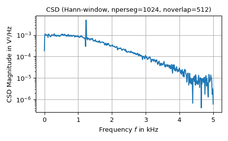
The following example plots the cross power spectral density of two signals with some common features:
import numpy as np from scipy import signal import matplotlib.pyplot as plt rng = np.random.default_rng() ... ... # Generate two test signals with some common features: N, fs = 100_000, 10e3 # number of samples and sampling frequency amp, freq = 20, 1234.0 # amplitude and frequency of utilized sine signal noise_power = 0.001 * fs / 2 time = np.arange(N) / fs b, a = signal.butter(2, 0.25, 'low') x = rng.normal(scale=np.sqrt(noise_power), size=time.shape) y = signal.lfilter(b, a, x) x += ampnp.sin(2np.pifreqtime) y += rng.normal(scale=0.1*np.sqrt(noise_power), size=time.shape) ... ... # Compute and plot the magnitude of the cross spectral density: nperseg, noverlap, win = 1024, 512, 'hann' f, Pxy = signal.csd(x, y, fs, win, nperseg, noverlap) fig0, ax0 = plt.subplots(tight_layout=True) ax0.set_title(f"CSD ({win.title()}-window, {nperseg=}, {noverlap=})") ax0.set(xlabel="Frequency fff in kHz", ylabel="CSD Magnitude in V²/Hz") ax0.semilogy(f/1e3, np.abs(Pxy)) ax0.grid() plt.show()
The cross spectral density is calculated by taking the average over the time slices of a spectrogram:
SFT = signal.ShortTimeFFT.from_window('hann', fs, nperseg, noverlap, ... scale_to='psd', fft_mode='onesided2X', ... phase_shift=None) Sxy1 = SFT.spectrogram(y, x, detr='constant', k_offset=nperseg//2, ... p0=0, p1=(N-noverlap) // SFT.hop) Pxy1 = Sxy1.mean(axis=-1) np.allclose(Pxy, Pxy1) # same result as with csd() True
As discussed in the Notes section, the results of using an approach analogous to the code snippet above and the csd function may deviate due to implementation details.
Note that the code snippet above can be easily adapted to determine other statistical properties than the mean value.