dbode — SciPy v1.15.3 Manual (original) (raw)
scipy.signal.
scipy.signal.dbode(system, w=None, n=100)[source]#
Calculate Bode magnitude and phase data of a discrete-time system.
Parameters:
system
An instance of the LTI class dlti or a tuple describing the system. The number of elements in the tuple determine the interpretation, i.e.:
(sys_dlti): Instance of LTI class dlti. Note that derived instances, such as instances of TransferFunction, ZerosPolesGain, or StateSpace, are allowed as well.(num, den, dt): Rational polynomial as described in TransferFunction. The coefficients of the polynomials should be specified in descending exponent order, e.g., z² + 3z + 5 would be represented as[1, 3, 5].(zeros, poles, gain, dt): Zeros, poles, gain form as described in ZerosPolesGain.(A, B, C, D, dt): State-space form as described in StateSpace.
warray_like, optional
Array of frequencies normalized to the Nyquist frequency being π, i.e., having unit radiant / sample. Magnitude and phase data is calculated for every value in this array. If not given, a reasonable set will be calculated.
nint, optional
Number of frequency points to compute if w is not given. The _n_frequencies are logarithmically spaced in an interval chosen to include the influence of the poles and zeros of the system.
Returns:
w1D ndarray
Array of frequencies normalized to the Nyquist frequency being np.pi/dtwith dt being the sampling interval of the system parameter. The unit is rad/s assuming dt is in seconds.
mag1D ndarray
Magnitude array in dB
phase1D ndarray
Phase array in degrees
Notes
This function is a convenience wrapper around dfreqresp for extracting magnitude and phase from the calculated complex-valued amplitude of the frequency response.
Added in version 0.18.0.
Examples
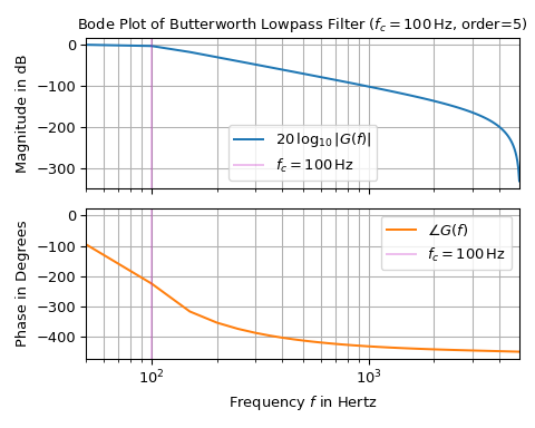
The following example shows how to create a Bode plot of a 5-th order Butterworth lowpass filter with a corner frequency of 100 Hz:
import matplotlib.pyplot as plt import numpy as np from scipy import signal ... T = 1e-4 # sampling interval in s f_c, o = 1e2, 5 # corner frequency in Hz (i.e., -3 dB value) and filter order bb, aa = signal.butter(o, f_c, 'lowpass', fs=1/T) ... w, mag, phase = signal.dbode((bb, aa, T)) w /= 2*np.pi # convert unit of frequency into Hertz ... fg, (ax0, ax1) = plt.subplots(2, 1, sharex='all', figsize=(5, 4), ... tight_layout=True) ax0.set_title("Bode Plot of Butterworth Lowpass Filter " + ... rf"($f_c={f_c:g},$Hz, order={o})") ax0.set_ylabel(r"Magnitude in dB") ax1.set(ylabel=r"Phase in Degrees", ... xlabel="Frequency fff in Hertz", xlim=(w[1], w[-1])) ax0.semilogx(w, mag, 'C0-', label=r"$20,\log_{10}|G(f)|$") # Magnitude plot ax1.semilogx(w, phase, 'C1-', label=r"$\angle G(f)$") # Phase plot ... for ax_ in (ax0, ax1): ... ax_.axvline(f_c, color='m', alpha=0.25, label=rf"${f_c=:g},$Hz") ... ax_.grid(which='both', axis='x') # plot major & minor vertical grid lines ... ax_.grid(which='major', axis='y') ... ax_.legend() plt.show()