genlaguerre — SciPy v1.15.3 Manual (original) (raw)
scipy.special.
scipy.special.genlaguerre(n, alpha, monic=False)[source]#
Generalized (associated) Laguerre polynomial.
Defined to be the solution of
\[x\frac{d^2}{dx^2}L_n^{(\alpha)} + (\alpha + 1 - x)\frac{d}{dx}L_n^{(\alpha)} + nL_n^{(\alpha)} = 0,\]
where \(\alpha > -1\); \(L_n^{(\alpha)}\) is a polynomial of degree \(n\).
Parameters:
nint
Degree of the polynomial.
alphafloat
Parameter, must be greater than -1.
monicbool, optional
If True, scale the leading coefficient to be 1. Default is_False_.
Returns:
Lorthopoly1d
Generalized Laguerre polynomial.
See also
Laguerre polynomial.
confluent hypergeometric function
Notes
For fixed \(\alpha\), the polynomials \(L_n^{(\alpha)}\)are orthogonal over \([0, \infty)\) with weight function\(e^{-x}x^\alpha\).
The Laguerre polynomials are the special case where \(\alpha = 0\).
References
[AS]
Milton Abramowitz and Irene A. Stegun, eds. Handbook of Mathematical Functions with Formulas, Graphs, and Mathematical Tables. New York: Dover, 1972.
Examples
The generalized Laguerre polynomials are closely related to the confluent hypergeometric function \({}_1F_1\):
\[L_n^{(\alpha)} = \binom{n + \alpha}{n} {}_1F_1(-n, \alpha +1, x)\]
This can be verified, for example, for \(n = \alpha = 3\) over the interval \([-1, 1]\):
import numpy as np from scipy.special import binom from scipy.special import genlaguerre from scipy.special import hyp1f1 x = np.arange(-1.0, 1.0, 0.01) np.allclose(genlaguerre(3, 3)(x), binom(6, 3) * hyp1f1(-3, 4, x)) True
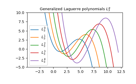
This is the plot of the generalized Laguerre polynomials\(L_3^{(\alpha)}\) for some values of \(\alpha\):
import matplotlib.pyplot as plt x = np.arange(-4.0, 12.0, 0.01) fig, ax = plt.subplots() ax.set_ylim(-5.0, 10.0) ax.set_title(r'Generalized Laguerre polynomials L3αL_3^{\alpha}L3α') for alpha in np.arange(0, 5): ... ax.plot(x, genlaguerre(3, alpha)(x), label=rf'$L_3^{(alpha)}$') plt.legend(loc='best') plt.show()