scipy.special.jv — SciPy v1.15.3 Manual (original) (raw)
scipy.special.jv(v, z, out=None) = <ufunc 'jv'>#
Bessel function of the first kind of real order and complex argument.
Parameters:
varray_like
Order (float).
zarray_like
Argument (float or complex).
outndarray, optional
Optional output array for the function values
Returns:
Jscalar or ndarray
Value of the Bessel function, \(J_v(z)\).
See also
\(J_v\) with leading exponential behavior stripped off.
spherical Bessel functions.
faster version of this function for order 0.
faster version of this function for order 1.
Notes
For positive v values, the computation is carried out using the AMOS[1] zbesj routine, which exploits the connection to the modified Bessel function \(I_v\),
\[ \begin{align}\begin{aligned}J_v(z) = \exp(v\pi\imath/2) I_v(-\imath z)\qquad (\Im z > 0)\\J_v(z) = \exp(-v\pi\imath/2) I_v(\imath z)\qquad (\Im z < 0)\end{aligned}\end{align} \]
For negative v values the formula,
\[J_{-v}(z) = J_v(z) \cos(\pi v) - Y_v(z) \sin(\pi v)\]
is used, where \(Y_v(z)\) is the Bessel function of the second kind, computed using the AMOS routine zbesy. Note that the second term is exactly zero for integer v; to improve accuracy the second term is explicitly omitted for v values such that v = floor(v).
Not to be confused with the spherical Bessel functions (see spherical_jn).
References
[1]
Donald E. Amos, “AMOS, A Portable Package for Bessel Functions of a Complex Argument and Nonnegative Order”,http://netlib.org/amos/
Examples
Evaluate the function of order 0 at one point.
from scipy.special import jv jv(0, 1.) 0.7651976865579666
Evaluate the function at one point for different orders.
jv(0, 1.), jv(1, 1.), jv(1.5, 1.) (0.7651976865579666, 0.44005058574493355, 0.24029783912342725)
The evaluation for different orders can be carried out in one call by providing a list or NumPy array as argument for the v parameter:
jv([0, 1, 1.5], 1.) array([0.76519769, 0.44005059, 0.24029784])
Evaluate the function at several points for order 0 by providing an array for z.
import numpy as np points = np.array([-2., 0., 3.]) jv(0, points) array([ 0.22389078, 1. , -0.26005195])
If z is an array, the order parameter v must be broadcastable to the correct shape if different orders shall be computed in one call. To calculate the orders 0 and 1 for an 1D array:
orders = np.array([[0], [1]]) orders.shape (2, 1)
jv(orders, points) array([[ 0.22389078, 1. , -0.26005195], [-0.57672481, 0. , 0.33905896]])
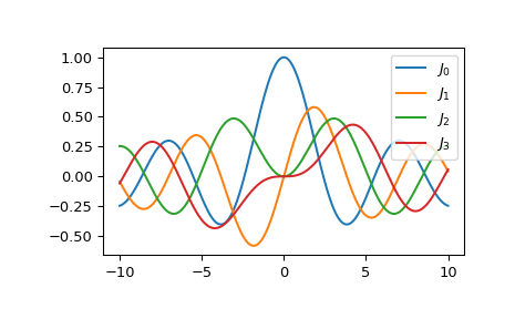
Plot the functions of order 0 to 3 from -10 to 10.
import matplotlib.pyplot as plt fig, ax = plt.subplots() x = np.linspace(-10., 10., 1000) for i in range(4): ... ax.plot(x, jv(i, x), label=f'$J_{i!r}$') ax.legend() plt.show()