scipy.special.stdtrit — SciPy v1.15.3 Manual (original) (raw)

scipy.special.stdtrit(df, p, out=None) = <ufunc 'stdtrit'>#

The _p_-th quantile of the student t distribution.

This function is the inverse of the student t distribution cumulative distribution function (CDF), returning t such that stdtr(df, t) = p.

Returns the argument t such that stdtr(df, t) is equal to p.

Parameters:

dfarray_like

Degrees of freedom

parray_like

Probability

outndarray, optional

Optional output array for the function results

Returns:

tscalar or ndarray

Value of t such that stdtr(df, t) == p

Notes

The student t distribution is also available as scipy.stats.t. Callingstdtrit directly can improve performance compared to the ppfmethod of scipy.stats.t (see last example below).

Examples

stdtrit represents the inverse of the student t distribution CDF which is available as stdtr. Here, we calculate the CDF for df atx=1. stdtrit then returns 1 up to floating point errors given the same value for df and the computed CDF value.

import numpy as np from scipy.special import stdtr, stdtrit import matplotlib.pyplot as plt df = 3 x = 1 cdf_value = stdtr(df, x) stdtrit(df, cdf_value) 0.9999999994418539

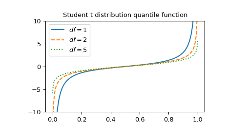
Plot the function for three different degrees of freedom.

x = np.linspace(0, 1, 1000) parameters = [(1, "solid"), (2, "dashed"), (5, "dotted")] fig, ax = plt.subplots() for (df, linestyle) in parameters: ... ax.plot(x, stdtrit(df, x), ls=linestyle, label=f"$df={df}$") ax.legend() ax.set_ylim(-10, 10) ax.set_title("Student t distribution quantile function") plt.show()

The function can be computed for several degrees of freedom at the same time by providing a NumPy array or list for df:

stdtrit([1, 2, 3], 0.7) array([0.72654253, 0.6172134 , 0.58438973])

It is possible to calculate the function at several points for several different degrees of freedom simultaneously by providing arrays for _df_and p with shapes compatible for broadcasting. Compute stdtrit at 4 points for 3 degrees of freedom resulting in an array of shape 3x4.

dfs = np.array([[1], [2], [3]]) p = np.array([0.2, 0.4, 0.7, 0.8]) dfs.shape, p.shape ((3, 1), (4,))

stdtrit(dfs, p) array([[-1.37638192, -0.3249197 , 0.72654253, 1.37638192], [-1.06066017, -0.28867513, 0.6172134 , 1.06066017], [-0.97847231, -0.27667066, 0.58438973, 0.97847231]])

The t distribution is also available as scipy.stats.t. Calling stdtritdirectly can be much faster than calling the ppf method ofscipy.stats.t. To get the same results, one must use the following parametrization: scipy.stats.t(df).ppf(x) = stdtrit(df, x).

from scipy.stats import t df, x = 3, 0.5 stdtrit_result = stdtrit(df, x) # this can be faster than below stats_result = t(df).ppf(x) stats_result == stdtrit_result # test that results are equal True