Scattered data interpolation (griddata) — SciPy v1.15.3 Manual (original) (raw)

Suppose you have multidimensional data, for instance, for an underlying function \(f(x, y)\) you only know the values at points (x[i], y[i])that do not form a regular grid.

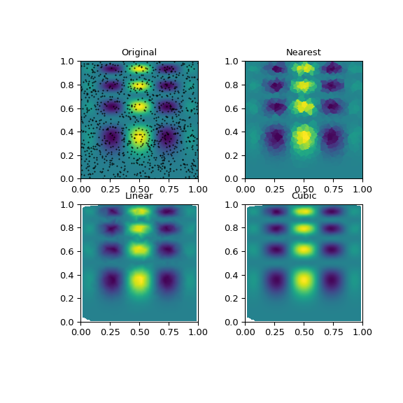
Suppose we want to interpolate the 2-D function

import numpy as np def func(x, y): ... return x*(1-x)np.cos(4np.pix) * np.sin(4np.pi*y**2)**2

on a grid in [0, 1]x[0, 1]

grid_x, grid_y = np.meshgrid(np.linspace(0, 1, 100), ... np.linspace(0, 1, 200), indexing='ij')

but we only know its values at 1000 data points:

rng = np.random.default_rng() points = rng.random((1000, 2)) values = func(points[:,0], points[:,1])

This can be done with griddata – below, we try out all of the interpolation methods:

from scipy.interpolate import griddata grid_z0 = griddata(points, values, (grid_x, grid_y), method='nearest') grid_z1 = griddata(points, values, (grid_x, grid_y), method='linear') grid_z2 = griddata(points, values, (grid_x, grid_y), method='cubic')

One can see that the exact result is reproduced by all of the methods to some degree, but for this smooth function the piecewise cubic interpolant gives the best results (black dots show the data being interpolated):

import matplotlib.pyplot as plt plt.subplot(221) plt.imshow(func(grid_x, grid_y).T, extent=(0, 1, 0, 1), origin='lower') plt.plot(points[:, 0], points[:, 1], 'k.', ms=1) # data plt.title('Original') plt.subplot(222) plt.imshow(grid_z0.T, extent=(0, 1, 0, 1), origin='lower') plt.title('Nearest') plt.subplot(223) plt.imshow(grid_z1.T, extent=(0, 1, 0, 1), origin='lower') plt.title('Linear') plt.subplot(224) plt.imshow(grid_z2.T, extent=(0, 1, 0, 1), origin='lower') plt.title('Cubic') plt.gcf().set_size_inches(6, 6) plt.show()

For each interpolation method, this function delegates to a corresponding class object — these classes can be used directly as well —NearestNDInterpolator, LinearNDInterpolator and CloughTocher2DInterpolatorfor piecewise cubic interpolation in 2D.

All these interpolation methods rely on triangulation of the data using theQHull library wrapped in scipy.spatial.

Note

griddata is based on triangulation, hence is appropriate for unstructured, scattered data. If your data is on a full grid, the griddata function — despite its name — is not the right tool. Use RegularGridInterpolatorinstead.

Note

If the input data is such that input dimensions have incommensurate units and differ by many orders of magnitude, the interpolant may have numerical artifacts. Consider rescaling the data before interpolating or use the rescale=True keyword argument to griddata.

Using radial basis functions for smoothing/interpolation#

Radial basis functions can be used for smoothing/interpolating scattered data in N dimensions, but should be used with caution for extrapolation outside of the observed data range.

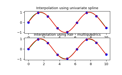
1-D Example#

This example compares the usage of the RBFInterpolator and UnivariateSplineclasses from the scipy.interpolate module.

import numpy as np from scipy.interpolate import RBFInterpolator, InterpolatedUnivariateSpline import matplotlib.pyplot as plt

setup data

x = np.linspace(0, 10, 9).reshape(-1, 1) y = np.sin(x) xi = np.linspace(0, 10, 101).reshape(-1, 1)

use fitpack2 method

ius = InterpolatedUnivariateSpline(x, y) yi = ius(xi)

fix, (ax1, ax2) = plt.subplots(2, 1) ax1.plot(x, y, 'bo') ax1.plot(xi, yi, 'g') ax1.plot(xi, np.sin(xi), 'r') ax1.set_title('Interpolation using univariate spline')

use RBF method

rbf = RBFInterpolator(x, y) fi = rbf(xi)

ax2.plot(x, y, 'bo') ax2.plot(xi, fi, 'g') ax2.plot(xi, np.sin(xi), 'r') ax2.set_title('Interpolation using RBF - multiquadrics') plt.tight_layout() plt.show()

2-D Example#

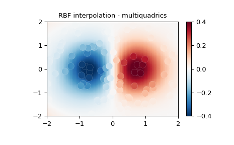
This example shows how to interpolate scattered 2-D data:

import numpy as np from scipy.interpolate import RBFInterpolator import matplotlib.pyplot as plt

2-d tests - setup scattered data

rng = np.random.default_rng() xy = rng.random((100, 2))*4.0-2.0 z = xy[:, 0]*np.exp(-xy[:, 0]**2-xy[:, 1]**2) edges = np.linspace(-2.0, 2.0, 101) centers = edges[:-1] + np.diff(edges[:2])[0] / 2. x_i, y_i = np.meshgrid(centers, centers) x_i = x_i.reshape(-1, 1) y_i = y_i.reshape(-1, 1) xy_i = np.concatenate([x_i, y_i], axis=1)

use RBF

rbf = RBFInterpolator(xy, z, epsilon=2) z_i = rbf(xy_i)

plot the result

fig, ax = plt.subplots() X_edges, Y_edges = np.meshgrid(edges, edges) lims = dict(cmap='RdBu_r', vmin=-0.4, vmax=0.4) mapping = ax.pcolormesh( ... X_edges, Y_edges, z_i.reshape(100, 100), ... shading='flat', **lims ... ) ax.scatter(xy[:, 0], xy[:, 1], 100, z, edgecolor='w', lw=0.1, **lims) ax.set( ... title='RBF interpolation - multiquadrics', ... xlim=(-2, 2), ... ylim=(-2, 2), ... ) fig.colorbar(mapping)