Multidimensional Image Processing (scipy.ndimage) — SciPy v1.15.3 Manual (original) (raw)
Introduction#
Image processing and analysis are generally seen as operations on 2-D arrays of values. There are, however, a number of fields where images of higher dimensionality must be analyzed. Good examples of these are medical imaging and biological imaging.numpy is suited very well for this type of applications due to its inherent multidimensional nature. The scipy.ndimagepackages provides a number of general image processing and analysis functions that are designed to operate with arrays of arbitrary dimensionality. The packages currently includes: functions for linear and non-linear filtering, binary morphology, B-spline interpolation, and object measurements.
Properties shared by all functions#
All functions share some common properties. Notably, all functions allow the specification of an output array with the _output_argument. With this argument, you can specify an array that will be changed in-place with the result with the operation. In this case, the result is not returned. Usually, using the output argument is more efficient, since an existing array is used to store the result.
The type of arrays returned is dependent on the type of operation, but it is, in most cases, equal to the type of the input. If, however, the output argument is used, the type of the result is equal to the type of the specified output argument. If no output argument is given, it is still possible to specify what the result of the output should be. This is done by simply assigning the desired numpy type object to the output argument. For example:
from scipy.ndimage import correlate import numpy as np correlate(np.arange(10), [1, 2.5]) array([ 0, 2, 6, 9, 13, 16, 20, 23, 27, 30]) correlate(np.arange(10), [1, 2.5], output=np.float64) array([ 0. , 2.5, 6. , 9.5, 13. , 16.5, 20. , 23.5, 27. , 30.5])
Filter functions#
The functions described in this section all perform some type of spatial filtering of the input array: the elements in the output are some function of the values in the neighborhood of the corresponding input element. We refer to this neighborhood of elements as the filter kernel, which is often rectangular in shape but may also have an arbitrary footprint. Many of the functions described below allow you to define the footprint of the kernel by passing a mask through the footprint parameter. For example, a cross-shaped kernel can be defined as follows:
footprint = np.array([[0, 1, 0], [1, 1, 1], [0, 1, 0]]) footprint array([[0, 1, 0], [1, 1, 1], [0, 1, 0]])
Usually, the origin of the kernel is at the center calculated by dividing the dimensions of the kernel shape by two. For instance, the origin of a 1-D kernel of length three is at the second element. Take, for example, the correlation of a 1-D array with a filter of length 3 consisting of ones:
from scipy.ndimage import correlate1d a = [0, 0, 0, 1, 0, 0, 0] correlate1d(a, [1, 1, 1]) array([0, 0, 1, 1, 1, 0, 0])
Sometimes, it is convenient to choose a different origin for the kernel. For this reason, most functions support the _origin_parameter, which gives the origin of the filter relative to its center. For example:
a = [0, 0, 0, 1, 0, 0, 0] correlate1d(a, [1, 1, 1], origin = -1) array([0, 1, 1, 1, 0, 0, 0])
The effect is a shift of the result towards the left. This feature will not be needed very often, but it may be useful, especially for filters that have an even size. A good example is the calculation of backward and forward differences:
a = [0, 0, 1, 1, 1, 0, 0] correlate1d(a, [-1, 1]) # backward difference array([ 0, 0, 1, 0, 0, -1, 0]) correlate1d(a, [-1, 1], origin = -1) # forward difference array([ 0, 1, 0, 0, -1, 0, 0])
We could also have calculated the forward difference as follows:
correlate1d(a, [0, -1, 1]) array([ 0, 1, 0, 0, -1, 0, 0])
However, using the origin parameter instead of a larger kernel is more efficient. For multidimensional kernels, origin can be a number, in which case the origin is assumed to be equal along all axes, or a sequence giving the origin along each axis.
Since the output elements are a function of elements in the neighborhood of the input elements, the borders of the array need to be dealt with appropriately by providing the values outside the borders. This is done by assuming that the arrays are extended beyond their boundaries according to certain boundary conditions. In the functions described below, the boundary conditions can be selected using the mode parameter, which must be a string with the name of the boundary condition. The following boundary conditions are currently supported:
mode description example “nearest” use the value at the boundary [1 2 3]->[1 1 2 3 3] “wrap” periodically replicate the array [1 2 3]->[3 1 2 3 1] “reflect” reflect the array at the boundary [1 2 3]->[1 1 2 3 3] “mirror” mirror the array at the boundary [1 2 3]->[2 1 2 3 2] “constant” use a constant value, default is 0.0 [1 2 3]->[0 1 2 3 0]
The following synonyms are also supported for consistency with the interpolation routines:
mode description “grid-constant” equivalent to “constant”* “grid-mirror” equivalent to “reflect” “grid-wrap” equivalent to “wrap”
* “grid-constant” and “constant” are equivalent for filtering operations, but have different behavior in interpolation functions. For API consistency, the filtering functions accept either name.
The “constant” mode is special since it needs an additional parameter to specify the constant value that should be used.
Note that modes mirror and reflect differ only in whether the sample at the boundary is repeated upon reflection. For mode mirror, the point of symmetry is exactly at the final sample, so that value is not repeated. This mode is also known as whole-sample symmetric since the point of symmetry falls on the final sample. Similarly, reflect is often referred to as half-sample symmetric as the point of symmetry is half a sample beyond the array boundary.
Note
The easiest way to implement such boundary conditions would be to copy the data to a larger array and extend the data at the borders according to the boundary conditions. For large arrays and large filter kernels, this would be very memory consuming, and the functions described below, therefore, use a different approach that does not require allocating large temporary buffers.
Correlation and convolution#
- The correlate1d function calculates a 1-D correlation along the given axis. The lines of the array along the given axis are correlated with the given weights. The _weights_parameter must be a 1-D sequence of numbers.
- The function correlate implements multidimensional correlation of the input array with a given kernel.
- The convolve1d function calculates a 1-D convolution along the given axis. The lines of the array along the given axis are convoluted with the given weights. The _weights_parameter must be a 1-D sequence of numbers.
- The function convolve implements multidimensional convolution of the input array with a given kernel.
Note
A convolution is essentially a correlation after mirroring the kernel. As a result, the origin parameter behaves differently than in the case of a correlation: the results is shifted in the opposite direction.
Smoothing filters#
- The gaussian_filter1d function implements a 1-D Gaussian filter. The standard deviation of the Gaussian filter is passed through the parameter sigma. Setting order = 0 corresponds to convolution with a Gaussian kernel. An order of 1, 2, or 3 corresponds to convolution with the first, second, or third derivatives of a Gaussian. Higher-order derivatives are not implemented.
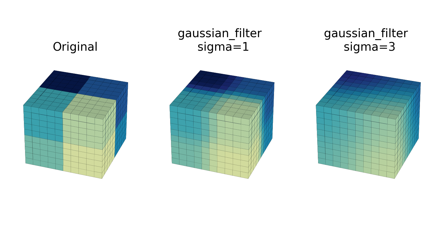
- The gaussian_filter function implements a multidimensional Gaussian filter. The standard deviations of the Gaussian filter along each axis are passed through the parameter sigma as a sequence or numbers. If sigma is not a sequence but a single number, the standard deviation of the filter is equal along all directions. The order of the filter can be specified separately for each axis. An order of 0 corresponds to convolution with a Gaussian kernel. An order of 1, 2, or 3 corresponds to convolution with the first, second, or third derivatives of a Gaussian. Higher-order derivatives are not implemented. The order parameter must be a number, to specify the same order for all axes, or a sequence of numbers to specify a different order for each axis. The example below shows the filter applied on test data with different values of sigma. The order parameter is kept at 0.
Note
The multidimensional filter is implemented as a sequence of 1-D Gaussian filters. The intermediate arrays are stored in the same data type as the output. Therefore, for output types with a lower precision, the results may be imprecise because intermediate results may be stored with insufficient precision. This can be prevented by specifying a more precise output type. - The uniform_filter1d function calculates a 1-D uniform filter of the given size along the given axis.
- The uniform_filter implements a multidimensional uniform filter. The sizes of the uniform filter are given for each axis as a sequence of integers by the size parameter. If size is not a sequence, but a single number, the sizes along all axes are assumed to be equal.
Note
The multidimensional filter is implemented as a sequence of 1-D uniform filters. The intermediate arrays are stored in the same data type as the output. Therefore, for output types with a lower precision, the results may be imprecise because intermediate results may be stored with insufficient precision. This can be prevented by specifying a more precise output type.
Filters based on order statistics#
- The minimum_filter1d function calculates a 1-D minimum filter of the given size along the given axis.
- The maximum_filter1d function calculates a 1-D maximum filter of the given size along the given axis.
- The minimum_filter function calculates a multidimensional minimum filter. Either the sizes of a rectangular kernel or the footprint of the kernel must be provided. The size parameter, if provided, must be a sequence of sizes or a single number, in which case the size of the filter is assumed to be equal along each axis. The footprint, if provided, must be an array that defines the shape of the kernel by its non-zero elements.
- The maximum_filter function calculates a multidimensional maximum filter. Either the sizes of a rectangular kernel or the footprint of the kernel must be provided. The size parameter, if provided, must be a sequence of sizes or a single number, in which case the size of the filter is assumed to be equal along each axis. The footprint, if provided, must be an array that defines the shape of the kernel by its non-zero elements.
- The rank_filter function calculates a multidimensional rank filter. The rank may be less than zero, i.e., rank = -1 indicates the largest element. Either the sizes of a rectangular kernel or the footprint of the kernel must be provided. The _size_parameter, if provided, must be a sequence of sizes or a single number, in which case the size of the filter is assumed to be equal along each axis. The footprint, if provided, must be an array that defines the shape of the kernel by its non-zero elements.
- The percentile_filter function calculates a multidimensional percentile filter. The percentile may be less than zero, i.e.,percentile = -20 equals percentile = 80. Either the sizes of a rectangular kernel or the footprint of the kernel must be provided. The size parameter, if provided, must be a sequence of sizes or a single number, in which case the size of the filter is assumed to be equal along each axis. The footprint, if provided, must be an array that defines the shape of the kernel by its non-zero elements.
- The median_filter function calculates a multidimensional median filter. Either the sizes of a rectangular kernel or the footprint of the kernel must be provided. The size parameter, if provided, must be a sequence of sizes or a single number, in which case the size of the filter is assumed to be equal along each axis. The footprint if provided, must be an array that defines the shape of the kernel by its non-zero elements.
Derivatives#
Derivative filters can be constructed in several ways. The functiongaussian_filter1d, described inSmoothing filters, can be used to calculate derivatives along a given axis using the order parameter. Other derivative filters are the Prewitt and Sobel filters:
- The prewitt function calculates a derivative along the given axis.
- The sobel function calculates a derivative along the given axis.
The Laplace filter is calculated by the sum of the second derivatives along all axes. Thus, different Laplace filters can be constructed using different second-derivative functions. Therefore, we provide a general function that takes a function argument to calculate the second derivative along a given direction.
- The function generic_laplace calculates a Laplace filter using the function passed through
derivative2to calculate second derivatives. The functionderivative2should have the following signature
derivative2(input, axis, output, mode, cval, *extra_arguments, **extra_keywords)
It should calculate the second derivative along the dimension_axis_. If output is notNone, it should use that for the output and returnNone, otherwise it should return the result. mode, cval have the usual meaning.
The extra_arguments and extra_keywords arguments can be used to pass a tuple of extra arguments and a dictionary of named arguments that are passed toderivative2at each call.
For exampledef d2(input, axis, output, mode, cval):
... return correlate1d(input, [1, -2, 1], axis, output, mode, cval, 0)
...
a = np.zeros((5, 5))
a[2, 2] = 1
from scipy.ndimage import generic_laplace
generic_laplace(a, d2)
array([[ 0., 0., 0., 0., 0.],
[ 0., 0., 1., 0., 0.],
[ 0., 1., -4., 1., 0.],
[ 0., 0., 1., 0., 0.],
[ 0., 0., 0., 0., 0.]])
To demonstrate the use of the extra_arguments argument, we could do
def d2(input, axis, output, mode, cval, weights):
... return correlate1d(input, weights, axis, output, mode, cval, 0,)
...
a = np.zeros((5, 5))
a[2, 2] = 1
generic_laplace(a, d2, extra_arguments = ([1, -2, 1],))
array([[ 0., 0., 0., 0., 0.],
[ 0., 0., 1., 0., 0.],
[ 0., 1., -4., 1., 0.],
[ 0., 0., 1., 0., 0.],
[ 0., 0., 0., 0., 0.]])
or
generic_laplace(a, d2, extra_keywords = {'weights': [1, -2, 1]})
array([[ 0., 0., 0., 0., 0.],
[ 0., 0., 1., 0., 0.],
[ 0., 1., -4., 1., 0.],
[ 0., 0., 1., 0., 0.],
[ 0., 0., 0., 0., 0.]])
The following two functions are implemented usinggeneric_laplace by providing appropriate functions for the second-derivative function:
- The function laplace calculates the Laplace using discrete differentiation for the second derivative (i.e., convolution with
[1, -2, 1]). - The function gaussian_laplace calculates the Laplace filter using gaussian_filter to calculate the second derivatives. The standard deviations of the Gaussian filter along each axis are passed through the parameter sigma as a sequence or numbers. If sigma is not a sequence but a single number, the standard deviation of the filter is equal along all directions.
The gradient magnitude is defined as the square root of the sum of the squares of the gradients in all directions. Similar to the generic Laplace function, there is a generic_gradient_magnitudefunction that calculates the gradient magnitude of an array.
- The function generic_gradient_magnitude calculates a gradient magnitude using the function passed through
derivativeto calculate first derivatives. The functionderivativeshould have the following signature
derivative(input, axis, output, mode, cval, *extra_arguments, **extra_keywords)
It should calculate the derivative along the dimension axis. If_output_ is notNone, it should use that for the output and returnNone, otherwise it should return the result. mode, cval have the usual meaning.
The extra_arguments and extra_keywords arguments can be used to pass a tuple of extra arguments and a dictionary of named arguments that are passed to derivative at each call.
For example, the sobel function fits the required signaturea = np.zeros((5, 5))
a[2, 2] = 1
from scipy.ndimage import sobel, generic_gradient_magnitude
generic_gradient_magnitude(a, sobel)
array([[ 0. , 0. , 0. , 0. , 0. ],
[ 0. , 1.41421356, 2. , 1.41421356, 0. ],
[ 0. , 2. , 0. , 2. , 0. ],
[ 0. , 1.41421356, 2. , 1.41421356, 0. ],
[ 0. , 0. , 0. , 0. , 0. ]])
See the documentation of generic_laplace for examples of using the extra_arguments and extra_keywords arguments.
The sobel and prewitt functions fit the required signature and can, therefore, be used directly withgeneric_gradient_magnitude.
- The function gaussian_gradient_magnitude calculates the gradient magnitude using gaussian_filter to calculate the first derivatives. The standard deviations of the Gaussian filter along each axis are passed through the parameter sigma as a sequence or numbers. If sigma is not a sequence but a single number, the standard deviation of the filter is equal along all directions.
Generic filter functions#
To implement filter functions, generic functions can be used that accept a callable object that implements the filtering operation. The iteration over the input and output arrays is handled by these generic functions, along with such details as the implementation of the boundary conditions. Only a callable object implementing a callback function that does the actual filtering work must be provided. The callback function can also be written in C and passed using aPyCapsule (see Extending scipy.ndimage in C for more information).
- The generic_filter1d function implements a generic 1-D filter function, where the actual filtering operation must be supplied as a python function (or other callable object). The generic_filter1d function iterates over the lines of an array and calls
functionat each line. The arguments that are passed tofunctionare 1-D arrays of thenumpy.float64type. The first contains the values of the current line. It is extended at the beginning and the end, according to the filter_size and origin arguments. The second array should be modified in-place to provide the output values of the line. For example, consider a correlation along one dimension:a = np.arange(12).reshape(3,4)
correlate1d(a, [1, 2, 3])
array([[ 3, 8, 14, 17],
[27, 32, 38, 41],
[51, 56, 62, 65]])
The same operation can be implemented using generic_filter1d, as follows:
def fnc(iline, oline):
... oline[...] = iline[:-2] + 2 * iline[1:-1] + 3 * iline[2:]
...
from scipy.ndimage import generic_filter1d
generic_filter1d(a, fnc, 3)
array([[ 3, 8, 14, 17],
[27, 32, 38, 41],
[51, 56, 62, 65]])
Here, the origin of the kernel was (by default) assumed to be in the middle of the filter of length 3. Therefore, each input line had been extended by one value at the beginning and at the end, before the function was called.
Optionally, extra arguments can be defined and passed to the filter function. The extra_arguments and extra_keywords arguments can be used to pass a tuple of extra arguments and/or a dictionary of named arguments that are passed to derivative at each call. For example, we can pass the parameters of our filter as an argument
def fnc(iline, oline, a, b):
... oline[...] = iline[:-2] + a * iline[1:-1] + b * iline[2:]
...
generic_filter1d(a, fnc, 3, extra_arguments = (2, 3))
array([[ 3, 8, 14, 17],
[27, 32, 38, 41],
[51, 56, 62, 65]])
or
generic_filter1d(a, fnc, 3, extra_keywords = {'a':2, 'b':3})
array([[ 3, 8, 14, 17],
[27, 32, 38, 41],
[51, 56, 62, 65]])
- The generic_filter function implements a generic filter function, where the actual filtering operation must be supplied as a python function (or other callable object). Thegeneric_filter function iterates over the array and calls
functionat each element. The argument offunctionis a 1-D array of thenumpy.float64type that contains the values around the current element that are within the footprint of the filter. The function should return a single value that can be converted to a double precision number. For example, consider a correlation:a = np.arange(12).reshape(3,4)
correlate(a, [[1, 0], [0, 3]])
array([[ 0, 3, 7, 11],
[12, 15, 19, 23],
[28, 31, 35, 39]])
The same operation can be implemented using generic_filter, as follows:
def fnc(buffer):
... return (buffer * np.array([1, 3])).sum()
...
from scipy.ndimage import generic_filter
generic_filter(a, fnc, footprint = [[1, 0], [0, 1]])
array([[ 0, 3, 7, 11],
[12, 15, 19, 23],
[28, 31, 35, 39]])
Here, a kernel footprint was specified that contains only two elements. Therefore, the filter function receives a buffer of length equal to two, which was multiplied with the proper weights and the result summed.
When calling generic_filter, either the sizes of a rectangular kernel or the footprint of the kernel must be provided. The size parameter, if provided, must be a sequence of sizes or a single number, in which case the size of the filter is assumed to be equal along each axis. The footprint, if provided, must be an array that defines the shape of the kernel by its non-zero elements.
Optionally, extra arguments can be defined and passed to the filter function. The extra_arguments and extra_keywords arguments can be used to pass a tuple of extra arguments and/or a dictionary of named arguments that are passed to derivative at each call. For example, we can pass the parameters of our filter as an argument
def fnc(buffer, weights):
... weights = np.asarray(weights)
... return (buffer * weights).sum()
...
generic_filter(a, fnc, footprint = [[1, 0], [0, 1]], extra_arguments = ([1, 3],))
array([[ 0, 3, 7, 11],
[12, 15, 19, 23],
[28, 31, 35, 39]])
or
generic_filter(a, fnc, footprint = [[1, 0], [0, 1]], extra_keywords= {'weights': [1, 3]})
array([[ 0, 3, 7, 11],
[12, 15, 19, 23],
[28, 31, 35, 39]])
These functions iterate over the lines or elements starting at the last axis, i.e., the last index changes the fastest. This order of iteration is guaranteed for the case that it is important to adapt the filter depending on spatial location. Here is an example of using a class that implements the filter and keeps track of the current coordinates while iterating. It performs the same filter operation as described above for generic_filter, but additionally prints the current coordinates:
a = np.arange(12).reshape(3,4)
class fnc_class: ... def init(self, shape): ... # store the shape: ... self.shape = shape ... # initialize the coordinates: ... self.coordinates = [0] * len(shape) ... ... def filter(self, buffer): ... result = (buffer * np.array([1, 3])).sum() ... print(self.coordinates) ... # calculate the next coordinates: ... axes = list(range(len(self.shape))) ... axes.reverse() ... for jj in axes: ... if self.coordinates[jj] < self.shape[jj] - 1: ... self.coordinates[jj] += 1 ... break ... else: ... self.coordinates[jj] = 0 ... return result ... fnc = fnc_class(shape = (3,4)) generic_filter(a, fnc.filter, footprint = [[1, 0], [0, 1]]) [0, 0] [0, 1] [0, 2] [0, 3] [1, 0] [1, 1] [1, 2] [1, 3] [2, 0] [2, 1] [2, 2] [2, 3] array([[ 0, 3, 7, 11], [12, 15, 19, 23], [28, 31, 35, 39]])
For the generic_filter1d function, the same approach works, except that this function does not iterate over the axis that is being filtered. The example for generic_filter1d then becomes this:
a = np.arange(12).reshape(3,4)
class fnc1d_class: ... def init(self, shape, axis = -1): ... # store the filter axis: ... self.axis = axis ... # store the shape: ... self.shape = shape ... # initialize the coordinates: ... self.coordinates = [0] * len(shape) ... ... def filter(self, iline, oline): ... oline[...] = iline[:-2] + 2 * iline[1:-1] + 3 * iline[2:] ... print(self.coordinates) ... # calculate the next coordinates: ... axes = list(range(len(self.shape))) ... # skip the filter axis: ... del axes[self.axis] ... axes.reverse() ... for jj in axes: ... if self.coordinates[jj] < self.shape[jj] - 1: ... self.coordinates[jj] += 1 ... break ... else: ... self.coordinates[jj] = 0 ... fnc = fnc1d_class(shape = (3,4)) generic_filter1d(a, fnc.filter, 3) [0, 0] [1, 0] [2, 0] array([[ 3, 8, 14, 17], [27, 32, 38, 41], [51, 56, 62, 65]])
Fourier domain filters#
The functions described in this section perform filtering operations in the Fourier domain. Thus, the input array of such a function should be compatible with an inverse Fourier transform function, such as the functions from the numpy.fft module. We, therefore, have to deal with arrays that may be the result of a real or a complex Fourier transform. In the case of a real Fourier transform, only half of the of the symmetric complex transform is stored. Additionally, it needs to be known what the length of the axis was that was transformed by the real fft. The functions described here provide a parameter n that, in the case of a real transform, must be equal to the length of the real transform axis before transformation. If this parameter is less than zero, it is assumed that the input array was the result of a complex Fourier transform. The parameter axis can be used to indicate along which axis the real transform was executed.
- The fourier_shift function multiplies the input array with the multidimensional Fourier transform of a shift operation for the given shift. The shift parameter is a sequence of shifts for each dimension or a single value for all dimensions.
- The fourier_gaussian function multiplies the input array with the multidimensional Fourier transform of a Gaussian filter with given standard deviations sigma. The sigma parameter is a sequence of values for each dimension or a single value for all dimensions.
- The fourier_uniform function multiplies the input array with the multidimensional Fourier transform of a uniform filter with given sizes size. The size parameter is a sequence of values for each dimension or a single value for all dimensions.
- The fourier_ellipsoid function multiplies the input array with the multidimensional Fourier transform of an elliptically-shaped filter with given sizes size. The size parameter is a sequence of values for each dimension or a single value for all dimensions. This function is only implemented for dimensions 1, 2, and 3.
Interpolation functions#
This section describes various interpolation functions that are based on B-spline theory. A good introduction to B-splines can be found in [1] with detailed algorithms for image interpolation given in [5].
Spline pre-filters#
Interpolation using splines of an order larger than 1 requires a pre-filtering step. The interpolation functions described in sectionInterpolation functions apply pre-filtering by callingspline_filter, but they can be instructed not to do this by setting the prefilter keyword equal to False. This is useful if more than one interpolation operation is done on the same array. In this case, it is more efficient to do the pre-filtering only once and use a pre-filtered array as the input of the interpolation functions. The following two functions implement the pre-filtering:
- The spline_filter1d function calculates a 1-D spline filter along the given axis. An output array can optionally be provided. The order of the spline must be larger than 1 and less than 6.
- The spline_filter function calculates a multidimensional spline filter.
Note
The multidimensional filter is implemented as a sequence of 1-D spline filters. The intermediate arrays are stored in the same data type as the output. Therefore, if an output with a limited precision is requested, the results may be imprecise because intermediate results may be stored with insufficient precision. This can be prevented by specifying a output type of high precision.
Interpolation boundary handling#
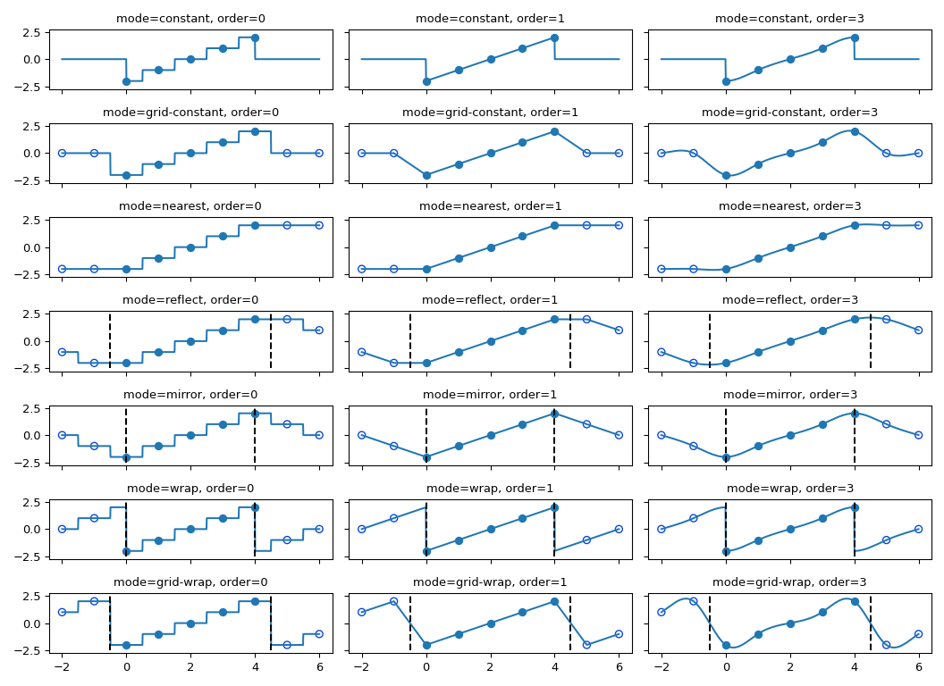
The interpolation functions all employ spline interpolation to effect some type of geometric transformation of the input array. This requires a mapping of the output coordinates to the input coordinates, and therefore, the possibility arises that input values outside the boundaries may be needed. This problem is solved in the same way as described in Filter functions for the multidimensional filter functions. Therefore, these functions all support a _mode_parameter that determines how the boundaries are handled, and a _cval_parameter that gives a constant value in case that the ‘constant’ mode is used. The behavior of all modes, including at non-integer locations is illustrated below. Note the boundaries are not handled the same for all modes;reflect (aka grid-mirror) and grid-wrap involve symmetry or repetition about a point that is half way between image samples (dashed vertical lines) while modes mirror and wrap treat the image as if it’s extent ends exactly at the first and last sample point rather than 0.5 samples past it.
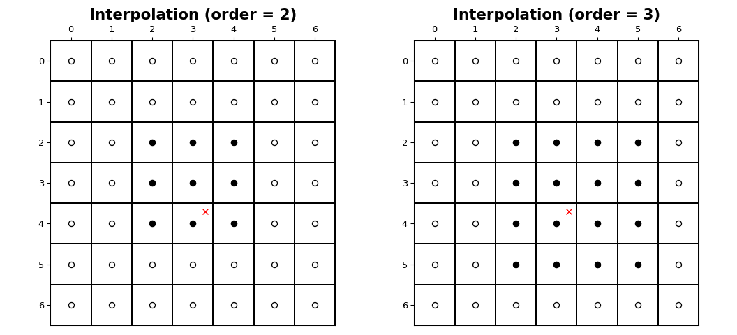
The coordinates of image samples fall on integer sampling locations in the range from 0 to shape[i] - 1 along each axis, i. The figure below illustrates the interpolation of a point at location (3.7, 3.3)within an image of shape (7, 7). For an interpolation of order n,n + 1 samples are involved along each axis. The filled circles illustrate the sampling locations involved in the interpolation of the value at the location of the red x.
Interpolation functions#
- The geometric_transform function applies an arbitrary geometric transform to the input. The given mapping function is called at each point in the output to find the corresponding coordinates in the input. mapping must be a callable object that accepts a tuple of length equal to the output array rank and returns the corresponding input coordinates as a tuple of length equal to the input array rank. The output shape and output type can optionally be provided. If not given, they are equal to the input shape and type.
For example:a = np.arange(12).reshape(4,3).astype(np.float64)
def shift_func(output_coordinates):
... return (output_coordinates[0] - 0.5, output_coordinates[1] - 0.5)
...
from scipy.ndimage import geometric_transform
geometric_transform(a, shift_func)
array([[ 0. , 0. , 0. ],
[ 0. , 1.3625, 2.7375],
[ 0. , 4.8125, 6.1875],
[ 0. , 8.2625, 9.6375]])
Optionally, extra arguments can be defined and passed to the filter function. The extra_arguments and extra_keywords arguments can be used to pass a tuple of extra arguments and/or a dictionary of named arguments that are passed to derivative at each call. For example, we can pass the shifts in our example as arguments
def shift_func(output_coordinates, s0, s1):
... return (output_coordinates[0] - s0, output_coordinates[1] - s1)
...
geometric_transform(a, shift_func, extra_arguments = (0.5, 0.5))
array([[ 0. , 0. , 0. ],
[ 0. , 1.3625, 2.7375],
[ 0. , 4.8125, 6.1875],
[ 0. , 8.2625, 9.6375]])
or
geometric_transform(a, shift_func, extra_keywords = {'s0': 0.5, 's1': 0.5})
array([[ 0. , 0. , 0. ],
[ 0. , 1.3625, 2.7375],
[ 0. , 4.8125, 6.1875],
[ 0. , 8.2625, 9.6375]])
- The function map_coordinates applies an arbitrary coordinate transformation using the given array of coordinates. The shape of the output is derived from that of the coordinate array by dropping the first axis. The parameter coordinates is used to find for each point in the output the corresponding coordinates in the input. The values of coordinates along the first axis are the coordinates in the input array at which the output value is found. (See also the numarray coordinates function.) Since the coordinates may be non- integer coordinates, the value of the input at these coordinates is determined by spline interpolation of the requested order.
Here is an example that interpolates a 2D array at(0.5, 0.5)and(1, 2):a = np.arange(12).reshape(4,3).astype(np.float64)
a
array([[ 0., 1., 2.],
[ 3., 4., 5.],
[ 6., 7., 8.],
[ 9., 10., 11.]])
from scipy.ndimage import map_coordinates
map_coordinates(a, [[0.5, 2], [0.5, 1]])
array([ 1.3625, 7.])
- The affine_transform function applies an affine transformation to the input array. The given transformation _matrix_and offset are used to find for each point in the output the corresponding coordinates in the input. The value of the input at the calculated coordinates is determined by spline interpolation of the requested order. The transformation matrix must be 2-D or can also be given as a 1-D sequence or array. In the latter case, it is assumed that the matrix is diagonal. A more efficient interpolation algorithm is then applied that exploits the separability of the problem. The output shape and output type can optionally be provided. If not given, they are equal to the input shape and type.
- The shift function returns a shifted version of the input, using spline interpolation of the requested order.
- The zoom function returns a rescaled version of the input, using spline interpolation of the requested order.
- The rotate function returns the input array rotated in the plane defined by the two axes given by the parameter axes, using spline interpolation of the requested order. The angle must be given in degrees. If reshape is true, then the size of the output array is adapted to contain the rotated input.
Morphology#
Binary morphology#
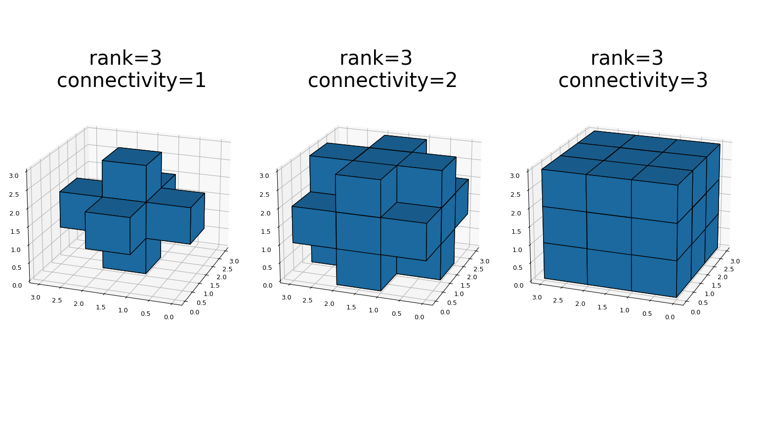
- The generate_binary_structure functions generates a binary structuring element for use in binary morphology operations. The_rank_ of the structure must be provided. The size of the structure that is returned is equal to three in each direction. The value of each element is equal to one if the square of the Euclidean distance from the element to the center is less than or equal to_connectivity_. For instance, 2-D 4-connected and 8-connected structures are generated as follows:
from scipy.ndimage import generate_binary_structure
generate_binary_structure(2, 1)
array([[False, True, False],
[ True, True, True],
[False, True, False]], dtype=bool)
generate_binary_structure(2, 2)
array([[ True, True, True],
[ True, True, True],
[ True, True, True]], dtype=bool)
This is a visual presentation of generate_binary_structure in 3D:
Most binary morphology functions can be expressed in terms of the basic operations erosion and dilation, which can be seen here:
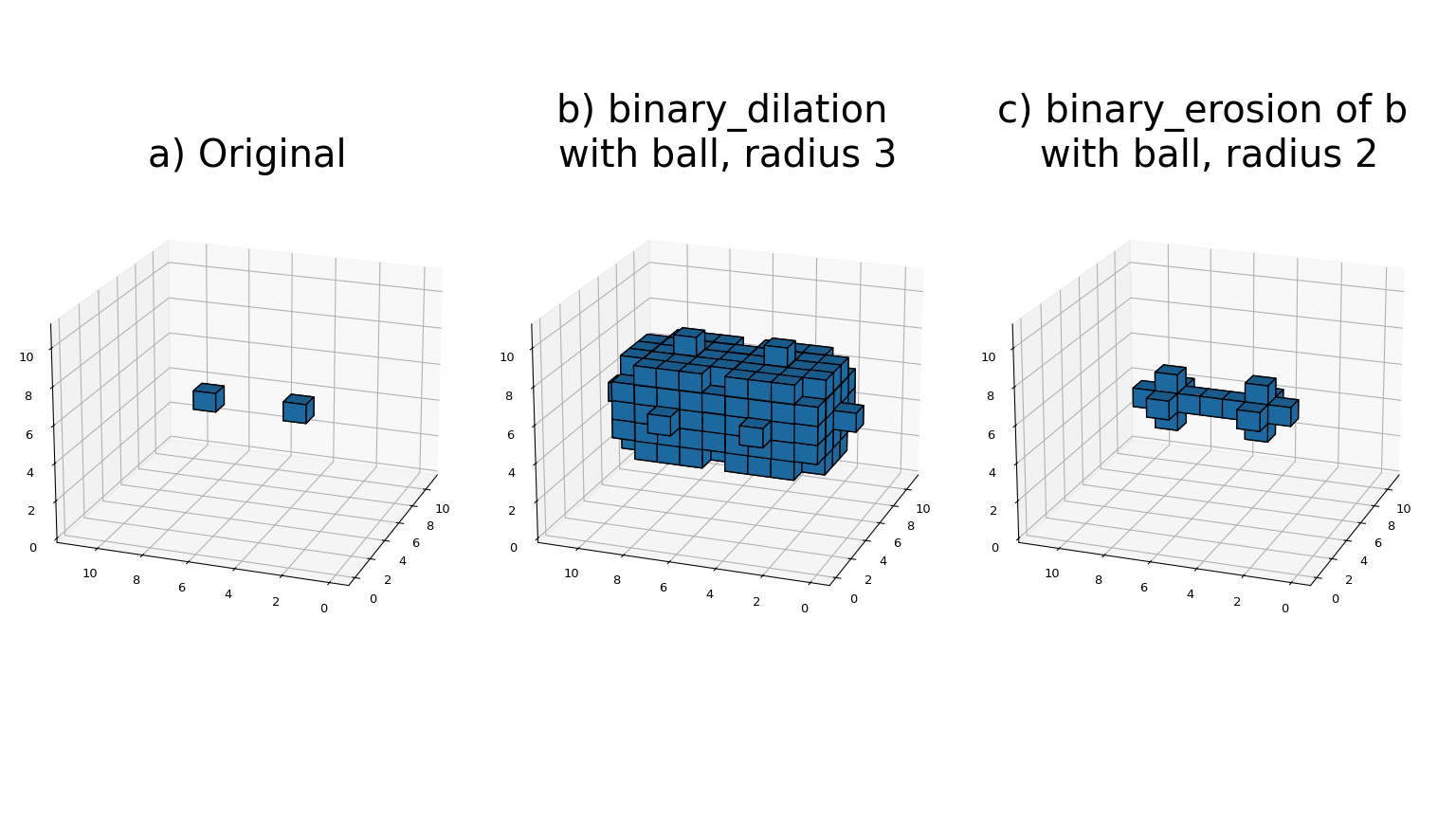
- The binary_erosion function implements binary erosion of arrays of arbitrary rank with the given structuring element. The origin parameter controls the placement of the structuring element, as described in Filter functions. If no structuring element is provided, an element with connectivity equal to one is generated using generate_binary_structure. The_border_value_ parameter gives the value of the array outside boundaries. The erosion is repeated iterations times. If_iterations_ is less than one, the erosion is repeated until the result does not change anymore. If a mask array is given, only those elements with a true value at the corresponding mask element are modified at each iteration.
- The binary_dilation function implements binary dilation of arrays of arbitrary rank with the given structuring element. The origin parameter controls the placement of the structuring element, as described in Filter functions. If no structuring element is provided, an element with connectivity equal to one is generated using generate_binary_structure. The_border_value_ parameter gives the value of the array outside boundaries. The dilation is repeated iterations times. If_iterations_ is less than one, the dilation is repeated until the result does not change anymore. If a mask array is given, only those elements with a true value at the corresponding mask element are modified at each iteration.
Here is an example of using binary_dilation to find all elements that touch the border, by repeatedly dilating an empty array from the border using the data array as the mask:
struct = np.array([[0, 1, 0], [1, 1, 1], [0, 1, 0]]) a = np.array([[1,0,0,0,0], [1,1,0,1,0], [0,0,1,1,0], [0,0,0,0,0]]) a array([[1, 0, 0, 0, 0], [1, 1, 0, 1, 0], [0, 0, 1, 1, 0], [0, 0, 0, 0, 0]]) from scipy.ndimage import binary_dilation binary_dilation(np.zeros(a.shape), struct, -1, a, border_value=1) array([[ True, False, False, False, False], [ True, True, False, False, False], [False, False, False, False, False], [False, False, False, False, False]], dtype=bool)
The binary_erosion and binary_dilation functions both have an iterations parameter, which allows the erosion or dilation to be repeated a number of times. Repeating an erosion or a dilation with a given structure n times is equivalent to an erosion or a dilation with a structure that is n-1 times dilated with itself. A function is provided that allows the calculation of a structure that is dilated a number of times with itself:
- The iterate_structure function returns a structure by dilation of the input structure iteration - 1 times with itself.
For instance:struct = generate_binary_structure(2, 1)
struct
array([[False, True, False],
[ True, True, True],
[False, True, False]], dtype=bool)
from scipy.ndimage import iterate_structure
iterate_structure(struct, 2)
array([[False, False, True, False, False],
[False, True, True, True, False],
[ True, True, True, True, True],
[False, True, True, True, False],
[False, False, True, False, False]], dtype=bool)
If the origin of the original structure is equal to 0, then it is
also equal to 0 for the iterated structure. If not, the origin
must also be adapted if the equivalent of the iterations
erosions or dilations must be achieved with the iterated
structure. The adapted origin is simply obtained by multiplying
with the number of iterations. For convenience, the
:func:iterate_structurealso returns the adapted origin if the
origin parameter is notNone:
.. code:: python
iterate_structure(struct, 2, -1)
(array([[False, False, True, False, False],
[False, True, True, True, False],
[ True, True, True, True, True],
[False, True, True, True, False],
[False, False, True, False, False]], dtype=bool), [-2, -2])
Other morphology operations can be defined in terms of erosion and dilation. The following functions provide a few of these operations for convenience:
- The binary_opening function implements binary opening of arrays of arbitrary rank with the given structuring element. Binary opening is equivalent to a binary erosion followed by a binary dilation with the same structuring element. The origin parameter controls the placement of the structuring element, as described inFilter functions. If no structuring element is provided, an element with connectivity equal to one is generated using generate_binary_structure. The iterations parameter gives the number of erosions that is performed followed by the same number of dilations.
- The binary_closing function implements binary closing of arrays of arbitrary rank with the given structuring element. Binary closing is equivalent to a binary dilation followed by a binary erosion with the same structuring element. The origin parameter controls the placement of the structuring element, as described inFilter functions. If no structuring element is provided, an element with connectivity equal to one is generated using generate_binary_structure. The iterations parameter gives the number of dilations that is performed followed by the same number of erosions.
- The binary_fill_holes function is used to close holes in objects in a binary image, where the structure defines the connectivity of the holes. The origin parameter controls the placement of the structuring element, as described inFilter functions. If no structuring element is provided, an element with connectivity equal to one is generated using generate_binary_structure.
- The binary_hit_or_miss function implements a binary hit-or-miss transform of arrays of arbitrary rank with the given structuring elements. The hit-or-miss transform is calculated by erosion of the input with the first structure, erosion of the logical not of the input with the second structure, followed by the logical and of these two erosions. The origin parameters control the placement of the structuring elements, as described inFilter functions. If origin2 equals
None, it is set equal to the origin1 parameter. If the first structuring element is not provided, a structuring element with connectivity equal to one is generated using generate_binary_structure. If_structure2_ is not provided, it is set equal to the logical _not_of structure1.
Grey-scale morphology#
Grey-scale morphology operations are the equivalents of binary morphology operations that operate on arrays with arbitrary values. Below, we describe the grey-scale equivalents of erosion, dilation, opening and closing. These operations are implemented in a similar fashion as the filters described in Filter functions, and we refer to this section for the description of filter kernels and footprints, and the handling of array borders. The grey-scale morphology operations optionally take a structure parameter that gives the values of the structuring element. If this parameter is not given, the structuring element is assumed to be flat with a value equal to zero. The shape of the structure can optionally be defined by the_footprint_ parameter. If this parameter is not given, the structure is assumed to be rectangular, with sizes equal to the dimensions of the structure array, or by the size parameter if structure is not given. The size parameter is only used if both structure and_footprint_ are not given, in which case the structuring element is assumed to be rectangular and flat with the dimensions given by_size_. The size parameter, if provided, must be a sequence of sizes or a single number in which case the size of the filter is assumed to be equal along each axis. The footprint parameter, if provided, must be an array that defines the shape of the kernel by its non-zero elements.
Similarly to binary erosion and dilation, there are operations for grey-scale erosion and dilation:
- The grey_erosion function calculates a multidimensional grey-scale erosion.
- The grey_dilation function calculates a multidimensional grey-scale dilation.
Grey-scale opening and closing operations can be defined similarly to their binary counterparts:
- The grey_opening function implements grey-scale opening of arrays of arbitrary rank. Grey-scale opening is equivalent to a grey-scale erosion followed by a grey-scale dilation.
- The grey_closing function implements grey-scale closing of arrays of arbitrary rank. Grey-scale opening is equivalent to a grey-scale dilation followed by a grey-scale erosion.
- The morphological_gradient function implements a grey-scale morphological gradient of arrays of arbitrary rank. The grey-scale morphological gradient is equal to the difference of a grey-scale dilation and a grey-scale erosion.
- The morphological_laplace function implements a grey-scale morphological laplace of arrays of arbitrary rank. The grey-scale morphological laplace is equal to the sum of a grey-scale dilation and a grey-scale erosion minus twice the input.
- The white_tophat function implements a white top-hat filter of arrays of arbitrary rank. The white top-hat is equal to the difference of the input and a grey-scale opening.
- The black_tophat function implements a black top-hat filter of arrays of arbitrary rank. The black top-hat is equal to the difference of a grey-scale closing and the input.
Distance transforms#
Distance transforms are used to calculate the minimum distance from each element of an object to the background. The following functions implement distance transforms for three different distance metrics: Euclidean, city block, and chessboard distances.
- The function distance_transform_cdt uses a chamfer type algorithm to calculate the distance transform of the input, by replacing each object element (defined by values larger than zero) with the shortest distance to the background (all non-object elements). The structure determines the type of chamfering that is done. If the structure is equal to ‘cityblock’, a structure is generated using generate_binary_structure with a squared distance equal to 1. If the structure is equal to ‘chessboard’, a structure is generated using generate_binary_structure with a squared distance equal to the rank of the array. These choices correspond to the common interpretations of the city block and the chessboard distance metrics in two dimensions.
In addition to the distance transform, the feature transform can be calculated. In this case, the index of the closest background element is returned along the first axis of the result. The_return_distances_, and return_indices flags can be used to indicate if the distance transform, the feature transform, or both must be returned.
The distances and indices arguments can be used to give optional output arrays that must be of the correct size and type (bothnumpy.int32). The basics of the algorithm used to implement this function are described in [2]. - The function distance_transform_edt calculates the exact Euclidean distance transform of the input, by replacing each object element (defined by values larger than zero) with the shortest Euclidean distance to the background (all non-object elements).
In addition to the distance transform, the feature transform can be calculated. In this case, the index of the closest background element is returned along the first axis of the result. The_return_distances_ and return_indices flags can be used to indicate if the distance transform, the feature transform, or both must be returned.
Optionally, the sampling along each axis can be given by the_sampling_ parameter, which should be a sequence of length equal to the input rank, or a single number in which the sampling is assumed to be equal along all axes.
The distances and indices arguments can be used to give optional output arrays that must be of the correct size and type (numpy.float64andnumpy.int32).The algorithm used to implement this function is described in [3]. - The function distance_transform_bf uses a brute-force algorithm to calculate the distance transform of the input, by replacing each object element (defined by values larger than zero) with the shortest distance to the background (all non-object elements). The metric must be one of “euclidean”, “cityblock”, or “chessboard”.
In addition to the distance transform, the feature transform can be calculated. In this case, the index of the closest background element is returned along the first axis of the result. The_return_distances_ and return_indices flags can be used to indicate if the distance transform, the feature transform, or both must be returned.
Optionally, the sampling along each axis can be given by the_sampling_ parameter, which should be a sequence of length equal to the input rank, or a single number in which the sampling is assumed to be equal along all axes. This parameter is only used in the case of the Euclidean distance transform.
The distances and indices arguments can be used to give optional output arrays that must be of the correct size and type (numpy.float64andnumpy.int32).
Note
This function uses a slow brute-force algorithm, the functiondistance_transform_cdt can be used to more efficiently calculate city block and chessboard distance transforms. The function distance_transform_edt can be used to more efficiently calculate the exact Euclidean distance transform.
Segmentation and labeling#
Segmentation is the process of separating objects of interest from the background. The most simple approach is, probably, intensity thresholding, which is easily done with numpy functions:
a = np.array([[1,2,2,1,1,0], ... [0,2,3,1,2,0], ... [1,1,1,3,3,2], ... [1,1,1,1,2,1]]) np.where(a > 1, 1, 0) array([[0, 1, 1, 0, 0, 0], [0, 1, 1, 0, 1, 0], [0, 0, 0, 1, 1, 1], [0, 0, 0, 0, 1, 0]])
The result is a binary image, in which the individual objects still need to be identified and labeled. The function labelgenerates an array where each object is assigned a unique number:
- The label function generates an array where the objects in the input are labeled with an integer index. It returns a tuple consisting of the array of object labels and the number of objects found, unless the output parameter is given, in which case only the number of objects is returned. The connectivity of the objects is defined by a structuring element. For instance, in 2D using a 4-connected structuring element gives:
a = np.array([[0,1,1,0,0,0],[0,1,1,0,1,0],[0,0,0,1,1,1],[0,0,0,0,1,0]])
s = [[0, 1, 0], [1,1,1], [0,1,0]]
from scipy.ndimage import label
label(a, s)
(array([[0, 1, 1, 0, 0, 0],
[0, 1, 1, 0, 2, 0],
[0, 0, 0, 2, 2, 2],
[0, 0, 0, 0, 2, 0]], dtype=int32), 2)
These two objects are not connected because there is no way in which we can place the structuring element, such that it overlaps with both objects. However, an 8-connected structuring element results in only a single object:
a = np.array([[0,1,1,0,0,0],[0,1,1,0,1,0],[0,0,0,1,1,1],[0,0,0,0,1,0]])
s = [[1,1,1], [1,1,1], [1,1,1]]
label(a, s)[0]
array([[0, 1, 1, 0, 0, 0],
[0, 1, 1, 0, 1, 0],
[0, 0, 0, 1, 1, 1],
[0, 0, 0, 0, 1, 0]], dtype=int32)
If no structuring element is provided, one is generated by callinggenerate_binary_structure (seeBinary morphology) using a connectivity of one (which in 2D is the 4-connected structure of the first example). The input can be of any type, any value not equal to zero is taken to be part of an object. This is useful if you need to ‘re-label’ an array of object indices, for instance, after removing unwanted objects. Just apply the label function again to the index array. For instance:
l, n = label([1, 0, 1, 0, 1])
l
array([1, 0, 2, 0, 3], dtype=int32)
l = np.where(l != 2, l, 0)
l
array([1, 0, 0, 0, 3], dtype=int32)
label(l)[0]
array([1, 0, 0, 0, 2], dtype=int32)
Note
The structuring element used by label is assumed to be symmetric.
There is a large number of other approaches for segmentation, for instance, from an estimation of the borders of the objects that can be obtained by derivative filters. One such approach is watershed segmentation. The function watershed_ift generates an array where each object is assigned a unique label, from an array that localizes the object borders, generated, for instance, by a gradient magnitude filter. It uses an array containing initial markers for the objects:
- The watershed_ift function applies a watershed from markers algorithm, using Image Foresting Transform, as described in[4].
- The inputs of this function are the array to which the transform is applied, and an array of markers that designate the objects by a unique label, where any non-zero value is a marker. For instance:
input = np.array([[0, 0, 0, 0, 0, 0, 0],
... [0, 1, 1, 1, 1, 1, 0],
... [0, 1, 0, 0, 0, 1, 0],
... [0, 1, 0, 0, 0, 1, 0],
... [0, 1, 0, 0, 0, 1, 0],
... [0, 1, 1, 1, 1, 1, 0],
... [0, 0, 0, 0, 0, 0, 0]], np.uint8)
markers = np.array([[1, 0, 0, 0, 0, 0, 0],
... [0, 0, 0, 0, 0, 0, 0],
... [0, 0, 0, 0, 0, 0, 0],
... [0, 0, 0, 2, 0, 0, 0],
... [0, 0, 0, 0, 0, 0, 0],
... [0, 0, 0, 0, 0, 0, 0],
... [0, 0, 0, 0, 0, 0, 0]], np.int8)
from scipy.ndimage import watershed_ift
watershed_ift(input, markers)
array([[1, 1, 1, 1, 1, 1, 1],
[1, 1, 2, 2, 2, 1, 1],
[1, 2, 2, 2, 2, 2, 1],
[1, 2, 2, 2, 2, 2, 1],
[1, 2, 2, 2, 2, 2, 1],
[1, 1, 2, 2, 2, 1, 1],
[1, 1, 1, 1, 1, 1, 1]], dtype=int8)
Here, two markers were used to designate an object (marker = 2) and the background (marker = 1). The order in which these are processed is arbitrary: moving the marker for the background to the lower-right corner of the array yields a different result:
markers = np.array([[0, 0, 0, 0, 0, 0, 0],
... [0, 0, 0, 0, 0, 0, 0],
... [0, 0, 0, 0, 0, 0, 0],
... [0, 0, 0, 2, 0, 0, 0],
... [0, 0, 0, 0, 0, 0, 0],
... [0, 0, 0, 0, 0, 0, 0],
... [0, 0, 0, 0, 0, 0, 1]], np.int8)
watershed_ift(input, markers)
array([[1, 1, 1, 1, 1, 1, 1],
[1, 1, 1, 1, 1, 1, 1],
[1, 1, 2, 2, 2, 1, 1],
[1, 1, 2, 2, 2, 1, 1],
[1, 1, 2, 2, 2, 1, 1],
[1, 1, 1, 1, 1, 1, 1],
[1, 1, 1, 1, 1, 1, 1]], dtype=int8)
The result is that the object (marker = 2) is smaller because the second marker was processed earlier. This may not be the desired effect if the first marker was supposed to designate a background object. Therefore, watershed_ift treats markers with a negative value explicitly as background markers and processes them after the normal markers. For instance, replacing the first marker by a negative marker gives a result similar to the first example:
markers = np.array([[0, 0, 0, 0, 0, 0, 0],
... [0, 0, 0, 0, 0, 0, 0],
... [0, 0, 0, 0, 0, 0, 0],
... [0, 0, 0, 2, 0, 0, 0],
... [0, 0, 0, 0, 0, 0, 0],
... [0, 0, 0, 0, 0, 0, 0],
... [0, 0, 0, 0, 0, 0, -1]], np.int8)
watershed_ift(input, markers)
array([[-1, -1, -1, -1, -1, -1, -1],
[-1, -1, 2, 2, 2, -1, -1],
[-1, 2, 2, 2, 2, 2, -1],
[-1, 2, 2, 2, 2, 2, -1],
[-1, 2, 2, 2, 2, 2, -1],
[-1, -1, 2, 2, 2, -1, -1],
[-1, -1, -1, -1, -1, -1, -1]], dtype=int8)
The connectivity of the objects is defined by a structuring element. If no structuring element is provided, one is generated by calling generate_binary_structure (seeBinary morphology) using a connectivity of one (which in 2D is a 4-connected structure.) For example, using an 8-connected structure with the last example yields a different object:
watershed_ift(input, markers,
... structure = [[1,1,1], [1,1,1], [1,1,1]])
array([[-1, -1, -1, -1, -1, -1, -1],
[-1, 2, 2, 2, 2, 2, -1],
[-1, 2, 2, 2, 2, 2, -1],
[-1, 2, 2, 2, 2, 2, -1],
[-1, 2, 2, 2, 2, 2, -1],
[-1, 2, 2, 2, 2, 2, -1],
[-1, -1, -1, -1, -1, -1, -1]], dtype=int8)
Note
The implementation of watershed_ift limits the data types of the input tonumpy.uint8andnumpy.uint16.
Object measurements#
Given an array of labeled objects, the properties of the individual objects can be measured. The find_objects function can be used to generate a list of slices that for each object, give the smallest sub-array that fully contains the object:
- The find_objects function finds all objects in a labeled array and returns a list of slices that correspond to the smallest regions in the array that contains the object.
For instance:a = np.array([[0,1,1,0,0,0],[0,1,1,0,1,0],[0,0,0,1,1,1],[0,0,0,0,1,0]])
l, n = label(a)
from scipy.ndimage import find_objects
f = find_objects(l)
a[f[0]]
array([[1, 1],
[1, 1]])
a[f[1]]
array([[0, 1, 0],
[1, 1, 1],
[0, 1, 0]])
The function find_objects returns slices for all objects, unless the max_label parameter is larger then zero, in which case only the first max_label objects are returned. If an index is missing in the label array,Noneis return instead of a slice. For example:
from scipy.ndimage import find_objects
find_objects([1, 0, 3, 4], max_label = 3)
[(slice(0, 1, None),), None, (slice(2, 3, None),)]
The list of slices generated by find_objects is useful to find the position and dimensions of the objects in the array, but can also be used to perform measurements on the individual objects. Say, we want to find the sum of the intensities of an object in image:
image = np.arange(4 * 6).reshape(4, 6) mask = np.array([[0,1,1,0,0,0],[0,1,1,0,1,0],[0,0,0,1,1,1],[0,0,0,0,1,0]]) labels = label(mask)[0] slices = find_objects(labels)
Then we can calculate the sum of the elements in the second object:
np.where(labels[slices[1]] == 2, image[slices[1]], 0).sum() 80
That is, however, not particularly efficient and may also be more complicated for other types of measurements. Therefore, a few measurements functions are defined that accept the array of object labels and the index of the object to be measured. For instance, calculating the sum of the intensities can be done by:
from scipy.ndimage import sum as ndi_sum ndi_sum(image, labels, 2) 80
For large arrays and small objects, it is more efficient to call the measurement functions after slicing the array:
ndi_sum(image[slices[1]], labels[slices[1]], 2) 80
Alternatively, we can do the measurements for a number of labels with a single function call, returning a list of results. For instance, to measure the sum of the values of the background and the second object in our example, we give a list of labels:
ndi_sum(image, labels, [0, 2]) array([178.0, 80.0])
The measurement functions described below all support the _index_parameter to indicate which object(s) should be measured. The default value of index is None. This indicates that all elements where the label is larger than zero should be treated as a single object and measured. Thus, in this case the labels array is treated as a mask defined by the elements that are larger than zero. If index is a number or a sequence of numbers it gives the labels of the objects that are measured. If index is a sequence, a list of the results is returned. Functions that return more than one result return their result as a tuple if index is a single number, or as a tuple of lists if index is a sequence.
- The sum function calculates the sum of the elements of the object with label(s) given by index, using the labels array for the object labels. If index is
None, all elements with a non-zero label value are treated as a single object. If label isNone, all elements of input are used in the calculation. - The mean function calculates the mean of the elements of the object with label(s) given by index, using the labels array for the object labels. If index is
None, all elements with a non-zero label value are treated as a single object. If label isNone, all elements of input are used in the calculation. - The variance function calculates the variance of the elements of the object with label(s) given by index, using the_labels_ array for the object labels. If index is
None, all elements with a non-zero label value are treated as a single object. If label isNone, all elements of input are used in the calculation. - The standard_deviation function calculates the standard deviation of the elements of the object with label(s) given by_index_, using the labels array for the object labels. If _index_is
None, all elements with a non-zero label value are treated as a single object. If label isNone, all elements of input are used in the calculation. - The minimum function calculates the minimum of the elements of the object with label(s) given by index, using the labels_array for the object labels. If index is
None, all elements with a non-zero label value are treated as a single object. If_label isNone, all elements of input are used in the calculation. - The maximum function calculates the maximum of the elements of the object with label(s) given by index, using the labels_array for the object labels. If index is
None, all elements with a non-zero label value are treated as a single object. If_label isNone, all elements of input are used in the calculation. - The minimum_position function calculates the position of the minimum of the elements of the object with label(s) given by_index_, using the labels array for the object labels. If _index_is
None, all elements with a non-zero label value are treated as a single object. If label isNone, all elements of input are used in the calculation. - The maximum_position function calculates the position of the maximum of the elements of the object with label(s) given by_index_, using the labels array for the object labels. If _index_is
None, all elements with a non-zero label value are treated as a single object. If label isNone, all elements of input are used in the calculation. - The extrema function calculates the minimum, the maximum, and their positions, of the elements of the object with label(s) given by index, using the labels array for the object labels. If_index_ is
None, all elements with a non-zero label value are treated as a single object. If label isNone, all elements of_input_ are used in the calculation. The result is a tuple giving the minimum, the maximum, the position of the minimum, and the position of the maximum. The result is the same as a tuple formed by the results of the functions minimum, maximum,minimum_position, and maximum_position that are described above. - The center_of_mass function calculates the center of mass of the object with label(s) given by index, using the labels_array for the object labels. If index is
None, all elements with a non-zero label value are treated as a single object. If_label isNone, all elements of input are used in the calculation. - The histogram function calculates a histogram of the object with label(s) given by index, using the labels array for the object labels. If index is
None, all elements with a non-zero label value are treated as a single object. If label isNone, all elements of input are used in the calculation. Histograms are defined by their minimum (min), maximum (max), and the number of bins (bins). They are returned as 1-D arrays of typenumpy.int32.
Extending scipy.ndimage in C#
A few functions in scipy.ndimage take a callback argument. This can be either a python function or a scipy.LowLevelCallable containing a pointer to a C function. Using a C function will generally be more efficient, since it avoids the overhead of calling a python function on many elements of an array. To use a C function, you must write a C extension that contains the callback function and a Python function that returns a scipy.LowLevelCallable containing a pointer to the callback.
An example of a function that supports callbacks isgeometric_transform, which accepts a callback function that defines a mapping from all output coordinates to corresponding coordinates in the input array. Consider the following python example, which uses geometric_transform to implement a shift function.
from scipy import ndimage
def transform(output_coordinates, shift): input_coordinates = output_coordinates[0] - shift, output_coordinates[1] - shift return input_coordinates
im = np.arange(12).reshape(4, 3).astype(np.float64) shift = 0.5 print(ndimage.geometric_transform(im, transform, extra_arguments=(shift,)))
We can also implement the callback function with the following C code:
/* example.c */
#include <Python.h> #include <numpy/npy_common.h>
static int _transform(npy_intp *output_coordinates, double *input_coordinates, int output_rank, int input_rank, void *user_data) { npy_intp i; double shift = *(double *)user_data;
for (i = 0; i < input_rank; i++) {
    input_coordinates[i] = output_coordinates[i] - shift;
}
return 1;
}
static char *transform_signature = "int (npy_intp *, double *, int, int, void *)";
static PyObject * py_get_transform(PyObject *obj, PyObject *args) { if (!PyArg_ParseTuple(args, "")) return NULL; return PyCapsule_New(_transform, transform_signature, NULL); }
static PyMethodDef ExampleMethods[] = { {"get_transform", (PyCFunction)py_get_transform, METH_VARARGS, ""}, {NULL, NULL, 0, NULL} };
/* Initialize the module */ static struct PyModuleDef example = { PyModuleDef_HEAD_INIT, "example", NULL, -1, ExampleMethods, NULL, NULL, NULL, NULL };
PyMODINIT_FUNC PyInit_example(void) { return PyModule_Create(&example); }
More information on writing Python extension modules can be foundhere. If the C code is in the file example.c, then it can be compiled after adding it to meson.build (see examples insidemeson.build files) and follow what’s there. After that is done, running the script:
import ctypes import numpy as np from scipy import ndimage, LowLevelCallable
from example import get_transform
shift = 0.5
user_data = ctypes.c_double(shift) ptr = ctypes.cast(ctypes.pointer(user_data), ctypes.c_void_p) callback = LowLevelCallable(get_transform(), ptr) im = np.arange(12).reshape(4, 3).astype(np.float64) print(ndimage.geometric_transform(im, callback))
produces the same result as the original python script.
In the C version, _transform is the callback function and the parameters output_coordinates and input_coordinates play the same role as they do in the python version, while output_rank andinput_rank provide the equivalents of len(output_coordinates)and len(input_coordinates). The variable shift is passed through user_data instead ofextra_arguments. Finally, the C callback function returns an integer status, which is one upon success and zero otherwise.
The function py_transform wraps the callback function in aPyCapsule. The main steps are:
- Initialize a PyCapsule. The first argument is a pointer to the callback function.
- The second argument is the function signature, which must match exactly the one expected by ndimage.
- Above, we used scipy.LowLevelCallable to specify
user_datathat we generated with ctypes.
A different approach would be to supply the data in the capsule context, that can be set by PyCapsule_SetContext and omit specifyinguser_datain scipy.LowLevelCallable. However, in this approach we would need to deal with allocation/freeing of the data — freeing the data after the capsule has been destroyed can be done by specifying a non-NULL callback function in the third argument of PyCapsule_New.
C callback functions for ndimage all follow this scheme. The next section lists the ndimage functions that accept a C callback function and gives the prototype of the function.
Below, we show alternative ways to write the code, using Numba, Cython,ctypes, or cffi instead of writing wrapper code in C.
Numba
Numba provides a way to write low-level functions easily in Python. We can write the above using Numba as:
example.py
import numpy as np import ctypes from scipy import ndimage, LowLevelCallable from numba import cfunc, types, carray
@cfunc(types.intc(types.CPointer(types.intp), types.CPointer(types.double), types.intc, types.intc, types.voidptr)) def transform(output_coordinates_ptr, input_coordinates_ptr, output_rank, input_rank, user_data): input_coordinates = carray(input_coordinates_ptr, (input_rank,)) output_coordinates = carray(output_coordinates_ptr, (output_rank,)) shift = carray(user_data, (1,), types.double)[0]
for i in range(input_rank):
    input_coordinates[i] = output_coordinates[i] - shift

return 1
shift = 0.5
Then call the function
user_data = ctypes.c_double(shift) ptr = ctypes.cast(ctypes.pointer(user_data), ctypes.c_void_p) callback = LowLevelCallable(transform.ctypes, ptr)
im = np.arange(12).reshape(4, 3).astype(np.float64) print(ndimage.geometric_transform(im, callback))
Cython
Functionally the same code as above can be written in Cython with somewhat less boilerplate as follows:
example.pyx
from numpy cimport npy_intp as intp
cdef api int transform(intp *output_coordinates, double *input_coordinates, int output_rank, int input_rank, void *user_data): cdef intp i cdef double shift = (<double *>user_data)[0]
for i in range(input_rank):
    input_coordinates[i] = output_coordinates[i] - shift
return 1
script.py
import ctypes import numpy as np from scipy import ndimage, LowLevelCallable
import example
shift = 0.5
user_data = ctypes.c_double(shift) ptr = ctypes.cast(ctypes.pointer(user_data), ctypes.c_void_p) callback = LowLevelCallable.from_cython(example, "transform", ptr) im = np.arange(12).reshape(4, 3).astype(np.float64) print(ndimage.geometric_transform(im, callback))
cffi
With cffi, you can interface with a C function residing in a shared library (DLL). First, we need to write the shared library, which we do in C — this example is for Linux/OSX:
/* example.c Needs to be compiled with "gcc -std=c99 -shared -fPIC -o example.so example.c" or similar */
#include <stdint.h>
int _transform(intptr_t *output_coordinates, double *input_coordinates, int output_rank, int input_rank, void *user_data) { int i; double shift = *(double *)user_data;
for (i = 0; i < input_rank; i++) {
    input_coordinates[i] = output_coordinates[i] - shift;
}
return 1;
}
The Python code calling the library is:
import os import numpy as np from scipy import ndimage, LowLevelCallable import cffi
Construct the FFI object, and copypaste the function declaration
ffi = cffi.FFI() ffi.cdef(""" int _transform(intptr_t *output_coordinates, double *input_coordinates, int output_rank, int input_rank, void *user_data); """)
Open library
lib = ffi.dlopen(os.path.abspath("example.so"))
Do the function call
user_data = ffi.new('double *', 0.5) callback = LowLevelCallable(lib._transform, user_data) im = np.arange(12).reshape(4, 3).astype(np.float64) print(ndimage.geometric_transform(im, callback))
You can find more information in the cffi documentation.
ctypes
With ctypes, the C code and the compilation of the so/DLL is as for cffi above. The Python code is different:
script.py
import os import ctypes import numpy as np from scipy import ndimage, LowLevelCallable
lib = ctypes.CDLL(os.path.abspath('example.so'))
shift = 0.5
user_data = ctypes.c_double(shift) ptr = ctypes.cast(ctypes.pointer(user_data), ctypes.c_void_p)
Ctypes has no built-in intptr type, so override the signature
instead of trying to get it via ctypes
callback = LowLevelCallable(lib._transform, ptr, "int _transform(intptr_t *, double *, int, int, void *)")
Perform the call
im = np.arange(12).reshape(4, 3).astype(np.float64) print(ndimage.geometric_transform(im, callback))
You can find more information in the ctypes documentation.