dsp.ColoredNoise - Generate colored noise signal - MATLAB (original) (raw)
Generate colored noise signal
Description
The dsp.ColoredNoise System object™ generates a colored noise signal with a power spectral density (PSD) of 1/|f|α over its entire frequency range. The inverse frequency power,α, can be any value in the interval [-2 2]. The type of colored noise the object generates depends on the Color you choose. When you set Color to 'custom', you can specify the power density of the noise through the InverseFrequencyPower property.
This object uses the default MATLAB® random stream, RandStream. Reset the default stream for repeatable simulations.
To generate colored noise signal:
- Create the
dsp.ColoredNoiseobject and set its properties. - Call the object with arguments, as if it were a function.
To learn more about how System objects work, see What Are System Objects?
Creation
Syntax
Description
`cn` = dsp.ColoredNoise creates a colored noise object, cn, that outputs a noise signal one sample or frame at a time, with a 1/|f|α spectral characteristic over its entire frequency range. Typical values for α are α = 1 (pink noise) and_α_ = 2 (brownian noise).
`cn` = dsp.ColoredNoise(`Name=Value`) creates a colored noise object and sets properties using one or more name-value arguments. For example, to specify the noise color as pink, set Color to "pink".
Example: dsp.ColoredNoise(Color='pink');
`cn` = dsp.ColoredNoise(pow,samp,numChan,`Name=Value`) creates a colored noise object with theInverseFrequencyPower property set to_pow_, the SamplesPerFrame property set to samp, and theNumChannels property set to_numChan_.
Example: dsp.ColoredNoise(1,44.1e3,1,OutputDataType='single');
`cn` = dsp.ColoredNoise(color,samp,numChan,`Name=Value`) creates a colored noise object with the Color property set to_color_, the SamplesPerFrame property set to_samp_, and the NumChannels property set to_numChan_.
Example:dsp.ColoredNoise('pink',1024,2,OutputDataType='single');
Properties
Unless otherwise indicated, properties are nontunable, which means you cannot change their values after calling the object. Objects lock when you call them, and therelease function unlocks them.
If a property is tunable, you can change its value at any time.
For more information on changing property values, seeSystem Design in MATLAB Using System Objects.
Noise color, specified as one of the following. Each color is associated with a specific inverse frequency power of the generated noise sequence.
"pink"–– The inverse frequency power_α_ equals 1."white"–– α = 0."brown"–– α = 2. Also known as red or Brownian noise."blue"–– α = -1. Also known as azure noise."purple"–– α = -2. Also known as violet noise."custom"–– For noise with a custom inverse frequency power, α equals the value of the InverseFrequencyPower property.InverseFrequencyPowerα can be any value in the interval [-2,2].
Data Types: char | string
Inverse frequency power α, specified as a real scalar in the interval [-2 2]. The inverse exponent defines the PSD of the random process as 1/|f|α. Values of InverseFrequencyPower greater than 0 generate lowpass noise with a singularity (pole) at f = 0. These processes exhibit long memory. Values of InverseFrequencyPower less than 0 generate highpass noise with increments that are negatively correlated. These processes are referred to as anti-persistent. Special cases include:
1–– Pink noise2–– Brown, red, or Brownian noise0–– White noise process with a flat PSD-1–– Blue or azure noise-2–– Purple of violet noise
In a log-log plot of power as a function of frequency, processes generated by this object exhibit an approximate linear relationship with slope equal to –α.
Dependencies
This property applies only when you set Color to "custom".
Data Types: single | double | int8 | int16 | int32 | int64 | uint8 | uint16 | uint32 | uint64
Source of the number of samples per frame, specified as"Property" or "Input port".
Data Types: char | string
Number of samples per output channel, specified as a positive integer. This property determines the number of rows in the generated signal.
Dependencies
To enable this property, setSamplesPerFrameSource to"Property".
Data Types: single | double | int8 | int16 | int32 | int64 | uint8 | uint16 | uint32 | uint64
Maximum number of samples per frame, specified as a positive integer.
The value you specify in the MaxSamplesPerFrame property acts as an upper limit to the number of samples in each frame that the object generates. If you specify a value greater than MaxSamplesPerFrame, the number of samples in each frame that the object generates equals the value in theMaxSamplesPerFrame property.
Dependencies
To enable this property, setSamplesPerFrameSource to "Input port".
Data Types: single | double | int8 | int16 | int32 | int64 | uint8 | uint16 | uint32 | uint64
Number of output channels, specified as an integer. This property determines the number of columns of the generated signal.
Data Types: single | double | int8 | int16 | int32 | int64 | uint8 | uint16 | uint32 | uint64
Source of the random number stream, specified as one of the following:
"Global stream"–– The current global random number stream is used for normally distributed random number generation."mt19937ar with seed"–– The mt19937ar algorithm is used for normally distributed random number generation. Theresetfunction reinitializes the random number stream to the value of theSeedproperty.
Data Types: char | string
Initial seed of mt19937ar random number stream generator algorithm, specified as a nonnegative integer. The reset function reinitializes the random number stream to the value of the Seed property.
Dependencies
This property applies only when you set theRandomStream property to"mt19937ar with seed".
Data Types: double
Specify the output to be bounded between +1 and −1, specified as:
true–– The internal random source that generates the noise is uniform instead of Gaussian, and a gain is applied so that the absolute maximum output never exceeds 1.
IfColoris set to"white", there is no color filter applied to the output of the random source. The output is uniform noise of amplitude between +1 and −1. The output distribution of filtered noise (such as pink noise) is quasi-Gaussian.
IfColoris set to any other option, then a coloring filter is applied to the output of the random source, followed by a gain which ensures that the absolute maximum output never exceeds1.false–– The internal random source is Gaussian. The output is not bounded.
Data Types: logical
Output data type, specified as either"double" or "single".
Data Types: char | string
Usage
Syntax
Description
[noiseOut](#d126e260681) = cn() outputs one sample or one frame of colored noise data.
[noiseOut](#d126e260681) = cn(`L`) outputs one frame of colored noise data of length L, whereL is a nonnegative integer.
This syntax applies only when you setSamplesPerFrameSource to "Input port".
Output Arguments
Object Functions
To use an object function, specify the System object as the first input argument. For example, to release system resources of a System object named obj, use this syntax:
| step | Run System object algorithm |
|---|---|
| release | Release resources and allow changes to System object property values and input characteristics |
| reset | Reset internal states of System object |
Examples
The output from this example shows that pink noise has approximately equal power in octave bands.
Generate a single-channel signal of pink noise that is 44,100 samples in length. Set the random number generator to the default settings for reproducible results.
pinkNoise = dsp.ColoredNoise(1,44.1e3,1)
pinkNoise = dsp.ColoredNoise with properties:
                Color: 'custom'
InverseFrequencyPower: 1
        BoundedOutput: false
          NumChannels: 1
SamplesPerFrameSource: 'Property'
      SamplesPerFrame: 44100
       OutputDataType: 'double'
         RandomStream: 'Global stream'
rng default; x = pinkNoise();
Set the sample rate to 44.1 kHz. Measure the power in octave bands beginning with 100-200 Hz and ending with 6.400-12.8 kHz. Display the results in a table.
beginfreq = 100; endfreq = 200; count = 1; freqinterval = zeros(7,2); Pwr = zeros(7,1); while(endfreq<=44.1e3/2) freqinterval(count,:) = [beginfreq endfreq]; Pwr(count) = bandpower(x,44.1e3,[beginfreq endfreq]); beginfreq = endfreq; endfreq = 2*endfreq; count = count+1; end Pwr = Pwr(:); table(freqinterval,Pwr)
ans=7×2 table
freqinterval Pwr
_____________ _______
 100      200    0.17549
 200      400    0.20313
 400      800     0.2438
 800     1600     0.2503
1600     3200    0.25233
3200     6400    0.26828
6400    12800    0.25211
The pink noise has roughly equal power in octave bands.
Rerun the preceding code with "InverseFrequencyPower" equal to 0, which generates a white noise signal. A white noise signal has a flat power spectral density, or equal power per unit frequency. Set the random number generator to the default settings for reproducible results.
whiteNoise = dsp.ColoredNoise(0,44.1e3,1); rng default; x = whiteNoise();
Set the sample rate to 44.1 kHz. Measure the power in octave bands beginning with 100-200 Hz and ending with 6.400-12.8 kHz. Display the results in a table.
beginfreq = 100; endfreq = 200; count = 1; while(endfreq<=44.1e3/2) freqinterval(count,:) = [beginfreq endfreq]; Pwr(count) = bandpower(x,44.1e3,[beginfreq endfreq]); beginfreq = endfreq; endfreq = 2*endfreq; count = count+1; end Pwr = Pwr(:); table(freqinterval,Pwr)
ans=7×2 table
freqinterval Pwr
_____________ _________
 100      200    0.0031417
 200      400    0.0073833
 400      800     0.017421
 800     1600     0.035926
1600     3200     0.071139
3200     6400      0.15183
6400    12800      0.28611
White noise has approximately equal power per unit frequency, so octave bands have an unequal distribution of power. Because the width of an octave band increases with increasing frequency, the power per octave band increases for white noise.
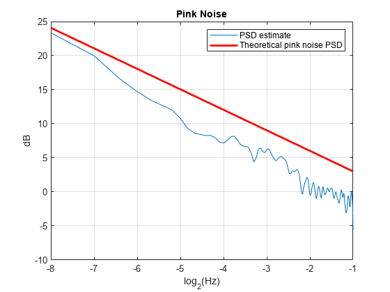
Generate a pink noise signal 2048 samples in length. The sample rate is 1 Hz. Obtain an estimate of the power spectral density using Welch's overlapped segment averaging.
cn = dsp.ColoredNoise("pink",SamplesPerFrame=2048); x = cn(); Fs = 1; [Pxx,F] = pwelch(x,hamming(128),[],[],Fs,"psd");
Construct the theoretical PSD of the pink noise process.
Display the Welch PSD estimate of the noise along with the theoretical PSD on a log-log plot. Plot the frequency axis with a base-2 logarithmic scale to clearly show the octaves. Plot the PSD estimate in dB, 10log10.
plot(log2(F(2:end)),10log10(Pxx(2:end))) hold on plot(log2(F(2:end)),10log10(PSDPink),"r",linewidth=2) xlabel("log_2(Hz)") ylabel("dB") title("Pink Noise") grid on legend("PSD estimate","Theoretical pink noise PSD") hold off
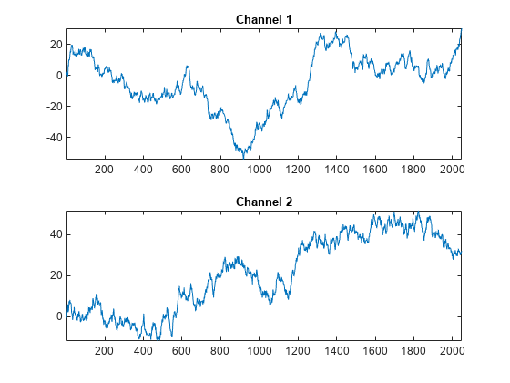
Generate two channels of Brownian noise by setting Color to "brown" and NumChannels to 2. Specify the number of samples in each frame as an input while running the object algorithm.
cn = dsp.ColoredNoise("brown",SamplesPerFrameSource="Input port",... NumChannels=2)
cn = dsp.ColoredNoise with properties:
                Color: 'brown'
        BoundedOutput: false
          NumChannels: 2
SamplesPerFrameSource: 'Input port'
   MaxSamplesPerFrame: 192000
       OutputDataType: 'double'
         RandomStream: 'Global stream'
x = cn(2048); subplot(2,1,1) plot(x(:,1)); title("Channel 1"); axis tight; subplot(2,1,2) plot(x(:,2)); title("Channel 2"); axis tight;
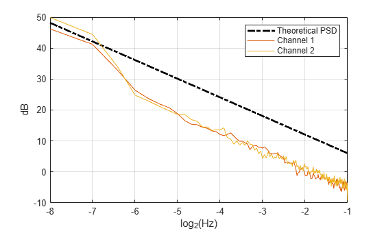
The sample rate is 1 Hz. Obtain Welch PSD estimates for both channels. The fourth argument of pwelch, NFFT, which is the number of FFT points, is empty. Hence, NFFT is set to 256. For even NFFT, The number of FFT points used to calculate the PSD estimate is (NFFT/2+1), which equals 129.
Fs = 1; Pxx = zeros(129,size(x,2)); for nn = 1:size(x,2) [Pxx(:,nn),F] = pwelch(x(:,nn),hamming(128),[],[],Fs,"psd"); end
Construct the theoretical PSD of a Brownian process. Plot the theoretical PSD along with both realizations on a log-log plot. Use a base-2 logarithmic scale for the frequency axis and plot the power spectral densities in dB.
PSDBrownian = 1./F(2:end).^2; figure; plot(log2(F(2:end)),10log10(PSDBrownian),"k-.",linewidth=2); hold on; plot(log2(F(2:end)),10log10(Pxx(2:end,:))); xlabel("log_2(Hz)"); ylabel("dB"); grid on; legend("Theoretical PSD","Channel 1", "Channel 2");
Note: The audioDeviceWriter System object™ is not supported in MATLAB Online.
This example shows how to stream in an audio file and add pink noise at a 0 dB signal-to-noise ratio (SNR). The example reads in frames of an audio file 1024 samples in length, measures the root mean square (RMS) value of the audio frame, and adds pink noise with the same RMS value as the audio frame.
Set up the System objects. Set "SamplesPerFrame" for both the file reader and the colored noise generator to 1024 samples. Set Color to "pink" to generate pink noise with a 1/|f| power spectral density.
N = 1024; afr = dsp.AudioFileReader(Filename="speech_dft.mp3",... SamplesPerFrame=N); adw = audioDeviceWriter(SampleRate=afr.SampleRate); cn = dsp.ColoredNoise("pink",SamplesPerFrame=N);
Stream the audio file in 1024 samples at a time. Measure the signal RMS value for each frame, generate a frame of pink noise equal in length, and scale the RMS value of the pink noise to match the signal. Add the scaled noise to the signal and play the output.
while ~isDone(afr)
audio = afr();
speechRMS = rms(audio);
noise = cn();
noiseRMS = rms(noise);
noise = noise*(speechRMS/noiseRMS);
sigPlusNoise = audio+noise;
adw(sigPlusNoise);
end
release(afr);
release(adw);
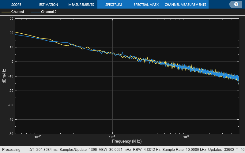
Generate two-channels of pink noise and compute the power density spectrum.
Set up the colored noise generator to generate two channels of pink noise with 1024 samples. Set up the spectrum analyzer to compute modified periodograms using a Hamming window and 50% overlap.
pinkNoise = dsp.ColoredNoise("pink",1024,2); sa = spectrumAnalyzer(SpectrumType="power-density",... Method="welch",... AveragingMethod="exponential",... ForgettingFactor=0.95,... OverlapPercent=50,Window="hamming",... PlotAsTwoSidedSpectrum=false, ... FrequencyScale="log",YLimits=[-50 30]);
Run the simulation for 30 seconds.
tic
while toc < 30
pink = pinkNoise();
sa(pink);
end
More About
Many phenomena in diverse fields, such as hydrology and finance, produce time series with PSD functions that follow a power law of the form
where α is a real number in the interval [-2,2] and L(f) is a positive, slowly-varying or constant function. Plotting the PSD of such processes on a log-log plot displays an approximate linear relationship between the log frequency and log PSD with slope equal to -α
It is often convenient to plot the PSD in dB as a function of the frequency on a base-2 logarithmic scale. The slope of the plot is then dB/octave. Rewriting the preceding equation, you obtain
with the slope in dB/octave given by
If α > 0, S(f) goes to infinity as the frequency, f, approaches 0. Stochastic processes with PSDs of this form exhibit long memory. Long-memory processes have autocorrelations that persist for a long time as opposed to decaying exponentially like many common time-series models. If α<0, the process is antipersistent and exhibits negative correlation between increments [1].
Special examples of 1|f|α processes include:
- α = 0 — White noise, where L(f) is a constant proportional to the process variance.
- α = 1 — Pink, or flicker noise. Pink noise has equal energy per octave. See Measure Pink Noise Power in Octave Bands for a demonstration. The power spectral density of pink noise decreases 3 dB per octave.
- α = 2 — brown noise, or Brownian motion. Brownian motion is a nonstationary process with stationary increments. You can think of Brownian motion as the integral of a white noise process. Even though Brownian motion is nonstationary, you can still define a generalized power spectrum, which behaves like 1|f|2. Accordingly, power in a brown noise decreases 6 dB per octave.
- α = −1 — blue noise. The power spectral density of blue noise increases 3 dB per octave.
- α = −2 — violet, or purple noise. The power spectral density of violet noise increases 6 dB per octave. You can think of violet noise as the derivative of white noise process.
Algorithms
The figure shows the overall process of generating the colored noise.

The random stream generator produces a stream of white noise that is either Gaussian or uniform in distribution. A coloring filter applied to the white noise generates colored noise with a power spectral density (PSD) function given by:
When α, the inverse frequency power, equals 0, no coloring filter is applied to the output of the random stream generator. If the bounded option is enabled, the output is uniform white noise with amplitude between +1 and −1. If the bounded output is not enabled, the output is a Gaussian white noise and the values are not bounded between +1 and −1. If α is set to any other value, then a coloring filter is applied to the output of the random stream generator. If the bounded output option is enabled, a gain_g_ is applied to the output of the coloring filter to ensure that the absolute maximum output never exceeds 1.
For details on colored noise processes and how the value of α affects the PSD of the colored noise, see Colored Noise Processes.
When the inverse frequency power α is positive, the colored noise is generated using an auto regressive (AR) model of order 63. The AR coefficients are:
Pink and brown noises are special cases, which are generated from specially tuned SOS filters of orders 12 and 10, respectively. These filters are optimized for better performance.
When the inverse frequency power α is negative, the colored noise is generated using a moving average (MA) model of order 255. The MA coefficients are:
Purple noise is generated from a first order filter, B = [1 −1].
The coloring filters applied (except pink, brown, and purple) are detailed on pp. 820–822 in[2].
References
[1] Beran, J., Y. Feng, S. Ghosh, and R. Kulik,Long-Memory Processes: Probabilistic Properties and Statistical Methods. NewYork: Springer, 2013.
[2] Kasdin, N.J. "Discrete Simulation of Colored Noise and Stochastic Processes and 1/fα Power Law Noise Generation."Proceedings of the IEEE®, Vol. 83, No. 5, 1995, pp. 802–827.
Extended Capabilities
Version History
Introduced in R2014a
Starting in R2022b, dsp.ColoredNoise object can generate colored noise signals of variable-sized output frames.
You can specify the frame size of the output colored noise signal as a nonnegative scalar value that is less than or equal to the MaxSamplesPerFrame property.