Random Source - Generate randomly distributed values - Simulink (original) (raw)
Generate randomly distributed values
Libraries:
DSP System Toolbox / Sources
Description
The Random Source block outputs a random signal with a uniform or Gaussian (normal) pseudorandom distribution. The block uses the Mersenne Twister random number generator to generate the sequence. The settings in the block dialog box determine the size, data type, and complexity of the signal.
The block can generate a single-channel or a multichannel signal.
Examples
Open the GenerateUniformSignal.slx model. The Random Source block in the model has the Distribution parameter set to Uniform. The minimum and maximum values of the uniform distribution are 1 and 3, respectively.
Set the Samples per frame parameter  to 512. The output random signal contains 512 samples in each channel (frame). Set the Sample time parameter
  to 0.1. Setting the Signal complexity to
 Real generates a real signal. Since the Initial seed parameter in the block dialog box is set to 1, the random signal that the block outputs is repeatable; that is, each time you simulate the model, the block generates the same pseudorandom sequence.
Run the model. The Random Source block generates a real single-channel signal with a uniform distribution. View the signal in the time scope.


The frame rate of the block MTs is  . View the frame rate in the timing legend.

Change the Sample time to 0.2 seconds and rerun the model. The output frame rate of the block is now  .
.

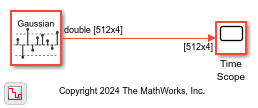
Open the GenerateGaussianSignal.slx model. The Random Source block in the model has the Distribution parameter set to Gaussian.
Generate Single-Channel Signal
Set the Mean and Variance parameters to 0 and 0.5, respectively. Because these values are scalars, the block generates a single-channel random signal. With the Samples per frame parameter set to 512, the block generates a 512-by-1 signal.


Generate Multichannel Signal
Set the Mean or Variance parameter to a row vector of four elements to generate a random signal with four channels. The value of the Mean parameter in this model is [0 2 4 6]. The Variance parameter must be a scalar or a row vector of four elements to match the dimensions of the Mean parameter. The value of the Variance parameter in this model is 0.5.
Run the model. The block generates a multichannel Gaussian random signal of size 512-by-4.

Use the Repeatability parameter to repeat the block output.
Open the RepeatRandomSignal.slx model. Set Repeatability to 'Specify Seed' to produce the same pseudorandom sequence each time you simulate the model. Specify the random seed as 123 through the Initial seed parameter.
Run the model.

Repeat the simulation and notice that the output values are exactly the same as the previous run.
2.3929    2.9615    1.8771
1.5723    2.3697    1.1194
1.4537    1.9619    1.7961
2.1026    1.7842    2.4760
2.4389    1.6864    1.3650
1.8462    2.4581    1.3509
Change the seed to 456 and run the model. The output values change but are exactly the same in subsequent simulations.
1.4975    2.7714    2.1514
1.3261    2.5182    1.2922
2.5673    1.3622    2.3732
2.6170    1.3003    1.9376
2.2513    1.8714    2.1400
2.2082    1.7705    2.2914
Set Repeatability to 'Not repeatable' and run the model.
2.8994    1.2989    2.5379
2.5772    2.5990    2.1492
2.7748    1.5675    2.9560
2.9537    1.4115    2.1808
1.3280    2.4491    1.9786
2.7592    2.3280    2.4437
Repeat the simulation. The output signal is now different compared to the previous run.
2.6861    2.7646    2.8339
1.9591    2.3445    2.0708
1.1533    1.8531    2.5022
1.9432    1.7436    2.7255
1.8130    1.5281    1.5712
2.9387    1.1459    2.5353
Generate a complex random signal by setting the Signal complexity parameter to Complex.
Open the ComplexRandomSignal model. The Distribution parameter in the Random Source block is set to Uniform. The minimum and maximum values of the uniform distribution are 1 and 3, respectively.
Run the model. The block generates a complex scalar random signal with a uniform distribution. The Complex to Real-Imag block splits the signal into real and imaginary components. Plot the data using the XY Graph block.


Change the distribution to Gaussian. Set the Mean parameter to a complex number. The real component of the Mean parameter specifies the mean of the real components in the channel, while the imaginary component specifies the mean of the imaginary components in the channel. If you omit the real or imaginary component from the Mean parameter, the block uses a default value of 0 as the mean of that component.
The variance must always be real and positive.

Select the Inherit via output port parameter to inherit the properties of the random signal through back propagation.
Open the InheritSignalProperties model. The model adds the outputs of the Random Source block and the Sine Wave block, and plots the resulting noisy sinusoidal signal in the time scope.
The Random Source block generates a random signal with a Gaussian distribution. The mean and variance of the distribution is 0 and 0.01, respectively.
Select the Inherit via output port parameter in the Random Source block. The block inherits the signal properties such as the size, data type, complexity, and sample time from the Sine Wave block via back propagation. The Sine Wave block generates a complex sinusoidal signal with a sample time of 0.001 seconds. The Random Source block inherits these properties and generates a random signal with the same properties.
Run the model. View the real and imaginary components of the noisy sinusoidal signal in the time scope.


This example shows how to use the Discrete Transfer Function Estimator block to estimate the frequency-domain transfer function of a system.
Open the ex_discretetransferfunctionestimator.slx model. The Random Source block generates the system input signal that you pass through the x port of the Discrete Transfer Function Estimator block. The sample rate of the input signal is 44.1 KHz. This input signal passes through a lowpass filter with a normalized cutoff frequency of 0.3. The filtered signal represents the system output signal that you input through the port y of the Discrete Transfer Function Estimator block. Because the Discrete Transfer Function Estimator block outputs complex values, compute the magnitude of the output signal to generate a plot of the transfer function estimate.
Run the model. The array plot shows the system transfer function, a lowpass filter that matches the frequency response of the Discrete FIR Filter block.
![]()
![]()
Extended Examples
Ports
Output
Signal of random values with uniform or Gaussian (normal) distribution. The settings in the block dialog box determine the size, data type, and complexity of the signal.
The block can generate a single-channel or a multichannel signal. TheSamples per frame parameter determines the number of samples in each channel (column) of the signal. TheOutput data type and Signal complexity parameters determine the data type and complexity of the signal.
Data Types: single | double
Complex Number Support: Yes
Parameters
Distribution Settings
Specify the distribution from which to draw the random values as one of these:
Uniform–– The block draws the output samples from a uniform distribution. You can specify the minimum and maximum values of the distribution using theMinimum andMaximum parameters, respectively. You can generate a complex number from the uniform distribution by setting the Signal complexity parameter toComplex.
All values in this [Minimum Maximum] range have an equal likelihood to be selected.
For an example, see Generate Random Signal with Uniform Distribution.Gaussian–– The block produces Gaussian random values by using the Ziggurat method. You can specify the mean and variance of the distribution using theMean and Variance parameters. You can generate a complex Gaussian signal by setting the Signal complexity parameter toComplex.
For an example, see Generate Random Signal with Gaussian Distribution.
Specify the minimum value in the uniform distribution as a scalar or a row vector of length N. When you specify a row vector, the block generates an _M_-by-N matrix containing a unique random distribution in each channel. M is the value you specify in the Samples per frame parameter.
For example, when you set Minimum to [0 0 -3 -3] and Maximum to [10 10 20 20], the block generates a four-channel output whose first and second columns contain random values in the range [0, 10], and whose third and fourth columns contain random values in the range [-3, 20].
The Minimum and Maximum values must be scalars or have the same number of columns. When you specify only one of theMinimum and Maximum parameters as a vector, the block expands the other parameter so that it is the same length as the vector.
Tunable: Yes
Dependencies
To enable this parameter, set Distribution toUniform.
Specify the maximum value in the uniform distribution as a scalar or a row vector of length N. When you specify a row vector, the block generates an _M_-by-N matrix containing a unique random distribution in each channel. M is the value you specify in the Samples per frame parameter.
For example, when you set Minimum to [0 0 -3 -3] and Maximum to [10 10 20 20], the block generates a four-channel output whose first and second columns contain random values in the range [0, 10], and whose third and fourth columns contain random values in the range [−3, 20].
The Minimum and Maximum values must be scalars or have the same number of columns. When you specify only one of theMinimum and Maximum parameters as a vector, the block expands the other parameter so it is the same length as the vector.
Tunable: Yes
Dependencies
To enable this parameter, set Distribution toUniform.
Specify the mean of the Gaussian (normal) distribution as a scalar or a row vector of length N. When you specify a row vector, the block generates an _M_-by-N matrix containing a distinct random distribution in each channel. M is the value you specify in the Samples per frame parameter.
The Mean and Variance values must be scalars or have the same number of columns. When you specify only one of theMean and Variance parameters as a vector, the block expands the other parameter so that it is the same length as the vector.
To generate a complex output signal with a Gaussian distribution, set Signal complexity toComplex and specify a complex value in theMean parameter. For more information, see theSignal complexity parameter description.
Tunable: Yes
Dependencies
To enable this parameter, set Distribution toGaussian.
Complex Number Support: Yes
Specify the variance of the Gaussian (normal) distribution as a scalar or a row vector of length N. When you specify a row vector, the block generates an _M_-by-N matrix containing a distinct random distribution in each channel. M is the value you specify in the Samples per frame parameter.
The Mean and Variance values must be scalars or have the same number of columns. When you specify only one of theMean and Variance parameters as a vector, the block expands the other parameter so that it is the same length as the vector.
To generate a complex output signal with a Gaussian distribution, the Variance parameter σ2 specifies the total variance for each output channel. This value is the sum of the variances of the real and imaginary components in that channel. For more information, see theSignal complexity parameter description.
Dependencies
To enable this parameter, set Distribution toGaussian.
Random Generator Settings
Option to repeat block output, specified as one of these:
Specify seed— The block uses the initial seed that you specify in the Initial seed parameter to produce a repeatable output for every simulation.Not repeatable— The block randomly selects an initial seed and produces a different pseudorandom sequence for every simulation.
For an example that shows the behavior of this parameter, see Repeat Random Signal Output.
Specify the initial seed(s) for the random number generator as a scalar. The generator produces an identical sequence of pseudorandom numbers each time you simulate the block with a particular initial seed.
Dependencies
To enable this parameter, set Repeatability toSpecify seed.
Signal Properties
When you select this check box, the block inherits the signal properties such as the samples per frame, output data type, signal complexity, and sample time from the downstream block and disables the corresponding parameters in the block dialog box. For an example, see Inherit Signal Properties Via Output Port.
Suppose that you want to back propagate a 1-D vector. The output of theRandom Source block is a 1-D vector of length_M_, where the block inherits the length_M_ from the downstream block. When theMinimum, Maximum,Mean, or Variance parameter specifies N channels, the 1-D vector output contains_M_/N samples from each channel. An error occurs in this case when M is not an integer multiple of N.
Suppose that you want to back propagate a M_-by-N signal. When N > 1, your signal has_N channels. When N =1, your signal has M channels. The value of the Minimum, Maximum,Mean, or Variance parameter can be a scalar or a vector of length equal to the number of channels. You can specify these parameters as row or column vectors, except when the signal is a row vector. In this case, you must specify theMinimum, Maximum,Mean, or Variance parameter as a row vector.
Specify the sample period _T_s of the random output sequence as a real positive scalar or -1. The output frame period is _MT_s.
If _T_s = −1, the block inherits the output sample period from its output port, but determines the dimensions and complexity of the signal from the block settings.
Dependencies
To enable this parameter, clear the Inherit via output port parameter.
Specify the number of samples M in each output frame as a positive integer. The output frame period is_MT_s, where_T_s is the value you specify in the Sample time parameter.
Dependencies
To enable this parameter, clear the Inherit via output port parameter.
Specify the complexity of the output as Real orComplex. These settings control all channels of the output. The real and complex components of the output are statistically independent.
For a complex output with a Uniform distribution, the block draws the real and imaginary components in each channel from the same uniform random distribution, defined by theMinimum and Maximum parameters for that channel.
For a complex output with a Gaussian distribution, the block draws the real and imaginary components in each channel from normal distributions with different means. In this case, theMean parameter for each channel must be a complex value. The real component of the Mean parameter specifies the mean of the real components in the channel, while the imaginary component specifies the mean of the imaginary components in the channel. When you omit the real or imaginary component from theMean parameter, the block uses a default value of 0 for the mean of that component.
For example, a Mean parameter setting of[5+2i 0.5 3i] generates a three-channel output with these mean values.
| Channel 1 mean | real = 5 | imaginary = 2 |
|---|---|---|
| Channel 2 mean | real = 0.5 | imaginary = 0 |
| Channel 3 mean | real = 0 | imaginary = 3 |
For a more detailed example, see Generate Complex Random Signal.
For a complex output, the Variance parameter σ2 specifies the total variance for each output channel. This value is the sum of the variances of the real and imaginary components in that channel.
The block divides the variance value you specify equally between the real and imaginary components.
Dependencies
To enable this parameter, clear the Inherit via output port parameter.
Specify the data type of the output as double precision or single precision.
Dependencies
To enable this parameter, clear the Inherit via output port parameter.
Specify the type of simulation to run. You can set this parameter to:
Interpreted execution–– Simulate model using the MATLAB® interpreter. This option shortens startup time.Code generation–– Simulate model using generated C code. The first time you run a simulation, Simulink generates C code for the block. The C code is reused for subsequent simulations as long as the model does not change. This option requires additional startup time but provides faster subsequent simulations.
Block Characteristics
| Data Types | double | single |
|---|---|
| Direct Feedthrough | no |
| Multidimensional Signals | no |
| Variable-Size Signals | no |
| Zero-Crossing Detection | no |
More About
Uniform distribution is a type of probability distribution in which all outcomes are equally likely.
Scalar Random Variable
Consider a scalar random variable X that the block draws from a uniform distribution U:
X ~ U([A,B_]), where_A and B are the minimum and maximum values of the distribution, respectively.
Alternatively, you can write X in terms of a scaled normalized uniform variable:
Uniform Random Vector
When you configure the block to have N > 1 channels, each output sample is a random vector of N independent entries. You can write_X_ as X:=[X1⋯XN], where Xk ~ U([Ak,_Bk_]) with {A1,…,AN} and {B1,…,BN} are the minimum and the maximum values of the vector parameters, respectively. When you setSamples per frame M > 1, each output frame is an_M_-by-N matrix of M independent uniform random row vectors.
Complex Uniform Random Variable
When you set the block to generate a complex scalar random variable, X := Y + j Z, where_Y_, Z ~ U([A, _B_]).
Alternatively, you can write X as
Complex Uniform Random Vector
When X is a vector of complex random variables, X:=[Y1+jZ1⋯YN+jZN], where Yk,Zk ~ U([Ak,_Bk_]) are all independent.
Scalar Random Variable
When you set the block to generate a random variable from a Gaussian (or normal) distribution, the variable X ~ N(μ,_σ_2), where μ and _σ_2 are the mean and variance values, respectively.
Alternatively, you can write X as X:=μ+σX˜, where X˜~N(0,1) is a standard normal variable.
Gaussian Random Vector
When you set the block to have N > 1 channels, each output sample is a random vector of N independent entries. When X is a Gaussian random vector, X:=[X1⋯XN], where Xk ~ N(μk,_σk_2), {_μ_1, …,μN} and {_σ_12, …,_σN_2} are the mean and variance values of N channels, respectively. The covariance matrix of the vector X is a diagonal matrix given by [σ12000⋱000σN2].
Complex Gaussian Random Variable
When you set the block to generate a complex scalar random variable, X := Y + j Z, where_Y_ ~ N(Re(μ),(_σ_2/2)) and Z ~ N(Im(μ),(_σ_2/2)) are independent. The mean value can be complex.
Alternatively, you can write X as X:=μ+σ2(Y˜+jZ˜).
Complex Gaussian Random Vector
When X is a vector of complex random variables, X:=[Y1+jZ1⋯YN+jZN], where Yk ~ N(Re(μk), (_σk_2/2)) and Zk ~ N(Im(μk), (_σk_2/2)) with {_μ_1, …,μN} and {_σ_12, …,_σN_2} are the mean and variance values of N channels, respectively.
Extended Capabilities
Version History
Introduced before R2006a
The Random Source block has been updated with these changes:
- Support for Mersenne Twister random number generator.
- The
Gaussiandistribution always uses the Zigguart method. TheSum of uniform valuesmethod is no longer supported. Repeatableoption is removed. To generate a repeatable output, set Repeatability toSpecify seed.- The initial seed must be a scalar. You can no longer specify a vector of seed values.
- When you specify an initial seed, the seed is no longer tunable, that is, you cannot change the value of the seed during simulation.
- The Sample mode parameter is removed. The sample mode of the block is now always discrete.
If you open a model saved in R2023b or a previous version of MATLAB, the model continues to use the older version of the block in R2024a. To use the updated version, obtain the Random Source block from theDSP System Toolbox/Sources library.