bubblelim - Map bubble sizes to data range - MATLAB (original) (raw)

Map bubble sizes to data range

Since R2020b

Syntax

Description

bubblelim([limits](#mw%5Fe146a04c-5d74-465e-b88b-fa095d38c104)) sets the bubble size limits for the current axes. Specify limits as a two-element vector of the form [bmin bmax], where bmax is greater than bmin. When you set the limits, the smallest bubble in the axes corresponds tobmin, and the largest bubble corresponds to bmax. For example, bubblelim([10 50]) maps the smallest and largest bubbles to the data values 10 and 50 respectively.

example

lim = bubblelim returns the bubble limits of the current axes as a two-element vector.

example

bubblelim([modevalue](#mw%5F1582ef4c-875d-4998-8e86-cfedf40fa2c9)) enables either automatic or manual mode for setting the limits. Specify modevalue as'auto' to let MATLAB® set the limits according to the range of your plotted data. Specify'manual' to hold the limits at the current value.

example

mv = bubblelim('mode') returns the current bubble limits mode value, which is either 'auto' or 'manual'. By default, the mode value is 'auto' unless you specify limits or set the mode value to 'manual'.

___ = bubblelim([ax](#mw%5Fabfb7e95-4068-4872-ad26-6508587b4814),___) sets the limits in the specified axes instead of the current axes. Specifyax before all other input arguments in any of the previous syntaxes. You can include an output argument if the original syntax supports an output argument. For example, lim = bubblelim(ax) returns the limits for the axesax.

example

Examples

collapse all

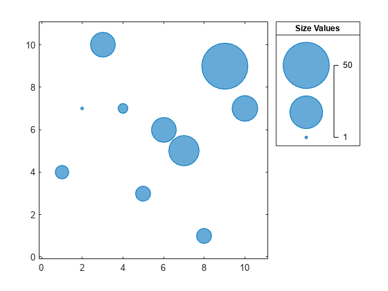
Create a bubble chart with a legend.

x = 1:10; y = [4 7 10 7 3 6 5 1 9 7]; sz = [5 1 14 6 9 12 15 20 8 2]; bubblechart(x,y,sz); bubblelegend('Size Values','Location','northeastoutside')

By default, the smallest and largest bubbles map to the smallest and largest values in the sz vector, respectively. Call the bubblelim function to get the current bubble limits.

Change the limits to [1 50]. As a result, the bubbles in the chart become smaller, and the labels in the bubble legend automatically update.

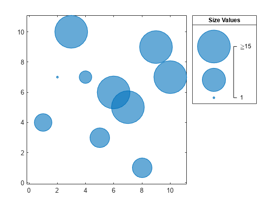
Create a bubble chart with a legend.

x = 1:10; y = [4 7 10 7 3 6 5 1 9 7]; sz = [5 1 15 3 6 15 22 6 50 16]; bubblechart(x,y,sz); bubblelegend('Size Values','Location','northeastoutside')

Get the current bubble limits.

Change the limits to [1 15]. As a result, some of the bubbles become larger, and any bubbles that have a sz value greater than 15 are clipped to the largest bubble size. The labels in the bubble legend automatically update.

When you create multiple bubble charts within the same axes, the bubble limits change for every bubble chart you add to the axes. They change to accommodate the sz values for all the charts. To hold the limits constant between plotting commands, use the bubblelim('manual') command.

For example, create a bubble chart with sz values that range from 1 to 20.

x = 1:10; y1 = [4 7 10 7 3 6 5 1 9 7]; sz1 = [5 1 14 6 9 12 15 20 8 2]; bubblechart(x,y1,sz1) hold on

Query the bubble limits.

Hold the bubble limits at their current value by calling the bubblelim('manual') command. Create another bubble chart in which the sz values range from 1 to 50.

bubblelim('manual') y2 = [10 7 2 3 8 9 2 1 3 4]; sz2 = [5 1 14 6 9 12 15 50 8 2]; bubblechart(x,y2,sz2);

Query the bubble limits again to verify that they have not changed.

Define two sets of data that show the contamination levels of a certain toxin across different towns on the east and west sides of a certain metropolitan area. Define towns1 and towns2 as the populations across the towns. Define nsites1 and nsites2 as the number of industrial sites in the corresponding towns. Then define levels1 and levels2 as the contamination levels in the towns.

towns1 = randi([25000 500000],[1 30]); towns2 = towns1/3; nsites1 = randi(10,1,30); nsites2 = randi(10,1,30); levels1 = (5 * nsites2) + (7 * randn(1,30) + 20); levels2 = (3 * nsites1) + (7 * randn(1,30) + 20);

Create a tiled chart layout so you can visualize the data side-by-side. Then create an axes object in the first tile and plot the data for the west side of the city. Add a title and axis labels. Then, repeat the process in the second tile to plot the east side data.

tiledlayout(1,2,'TileSpacing','compact')

% West side ax1 = nexttile; bubblechart(ax1,nsites1,levels1,towns1); title('West Side') xlabel('Number of Industrial Sites')

% East side ax2 = nexttile; bubblechart(ax2,nsites2,levels2,towns2); title('East Side') xlabel('Number of Industrial Sites') ylabel('Contamination Level')

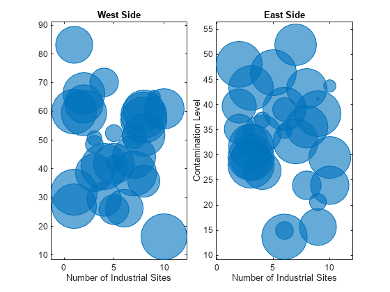
Reduce all the bubble sizes to make it easier to see all the bubbles. In this case, change the range of diameters to be between 5 and 30 points.

bubblesize(ax1,[5 30]) bubblesize(ax2,[5 30])

The west side towns are three times the size of the east side towns, but the bubble sizes do not reflect this information in the preceding charts. This is because the smallest and largest bubbles map to the smallest and largest data points in each of the axes. To display the bubbles on the same scale, define a vector called alltowns that includes the populations from both sides of the city. Use the bubblelim function to reset the scaling for both charts. Next, use the xlim and ylim functions to display the charts with the same _x_- and _y_-axis limits.

% Adjust scale of the bubbles alltowns = [towns1 towns2]; newlims = [min(alltowns) max(alltowns)]; bubblelim(ax1,newlims) bubblelim(ax2,newlims)

% Adjust x-axis limits allx = [xlim(ax1) xlim(ax2)]; xmin = min(allx); xmax = max(allx); xlim([ax1 ax2],[xmin xmax]);

% Adjust y-axis limits ally = [ylim(ax1) ylim(ax2)]; ymin = min(ally); ymax = max(ally); ylim([ax1 ax2],[ymin ymax]);

Input Arguments

collapse all

Data limits, specified as a two-element vector where the first element is less than the second.

Example: bubblelim([10 50]) maps the smallest and largest bubbles to the data values 10 and 50 respectively.

Mode value, specified as one of these values:

• 'auto' — Enables MATLAB to determine the bubble limits. The limits span the range of the plotted data. Use this option if you change the limits and then want to set them back to the default values.
• 'manual' — Keeps the limits at the current values. Use this option if you want to retain the current limits when adding new data to the axes using the hold on command.

Target axes, specified as an Axes, PolarAxes, or GeographicAxes object.

Version History

Introduced in R2020b