eigs - Subset of eigenvalues and eigenvectors - MATLAB (original) (raw)
Subset of eigenvalues and eigenvectors
Syntax
Description
[d](#bu2%5Fq3e-d) = eigs([A](#bu2%5Fq3e-A)) returns a vector of the six largest magnitude eigenvalues of matrix A. This is most useful when computing all of the eigenvalues with eig is computationally expensive, such as with large sparse matrices.
[d](#bu2%5Fq3e-d) = eigs([A](#bu2%5Fq3e-A),[k](#bu2%5Fq3e-k)) returns the k largest magnitude eigenvalues.
[d](#bu2%5Fq3e-d) = eigs([A](#bu2%5Fq3e-A),[k](#bu2%5Fq3e-k),[sigma](#bu2%5Fq3e-sigma)) returns k eigenvalues based on the value ofsigma. For example,eigs(A,k,'smallestabs') returns the k smallest magnitude eigenvalues.
[d](#bu2%5Fq3e-d) = eigs([A](#bu2%5Fq3e-A),[k](#bu2%5Fq3e-k),[sigma](#bu2%5Fq3e-sigma),[Name,Value](#namevaluepairarguments)) specifies additional options with one or more name-value pair arguments. For example, eigs(A,k,sigma,'Tolerance',1e-3) adjusts the convergence tolerance for the algorithm.
[d](#bu2%5Fq3e-d) = eigs([A](#bu2%5Fq3e-A),[k](#bu2%5Fq3e-k),[sigma](#bu2%5Fq3e-sigma),[opts](#bu2%5Fq3e-opts)) specifies options using a structure.
[d](#bu2%5Fq3e-d) = eigs([A](#bu2%5Fq3e-A),[B](#bu2%5Fq3e-B),___) solves the generalized eigenvalue problem A*V = B*V*D. You can optionally specify k, sigma,opts, or name-value pairs as additional input arguments.
[d](#bu2%5Fq3e-d) = eigs([Afun](#bu2%5Fq3e-Afun),[n](#bu2%5Fq3e-n),___) specifies a function handle Afun instead of a matrix. The second input n gives the size of matrix A used in Afun. You can optionally specifyB, k, sigma,opts, or name-value pairs as additional input arguments.
[[V](#bu2%5Fq3e-V),[D](#bu2%5Fq3e-D)] = eigs(___) returns diagonal matrix D containing the eigenvalues on the main diagonal, and matrix V whose columns are the corresponding eigenvectors. You can use any of the input argument combinations in previous syntaxes.
[[V](#bu2%5Fq3e-V),[D](#bu2%5Fq3e-D),[flag](#bu2%5Fq3e-flag)] = eigs(___) also returns a convergence flag. If flag is 0, then all the eigenvalues converged.
Examples
The matrix A = delsq(numgrid('C',15)) is a symmetric positive definite matrix with eigenvalues reasonably well-distributed in the interval (0 8). Compute the six largest magnitude eigenvalues.
A = delsq(numgrid('C',15)); d = eigs(A)
d = 6×1
7.8666
7.7324
7.6531
7.5213
7.4480
7.3517
Specify a second input to compute a specific number of the largest eigenvalues.
d = 3×1
7.8666
7.7324
7.6531
The matrix A = delsq(numgrid('C',15)) is a symmetric positive definite matrix with eigenvalues reasonably well-distributed in the interval (0 8). Compute the five smallest eigenvalues.
A = delsq(numgrid('C',15));
d = eigs(A,5,'smallestabs')
d = 5×1
0.1334
0.2676
0.3469
0.4787
0.5520
Create a 1500-by-1500 random sparse matrix with a 25% approximate density of nonzero elements.
n = 1500; A = sprand(n,n,0.25);
Find the LU factorization of the matrix, returning a permutation vector p that satisfies A(p,:) = L*U.
[L,U,p] = lu(A,'vector');
Create a function handle Afun that accepts a vector input x and uses the results of the LU decomposition to, in effect, return A\x.
Afun = @(x) U(L(x(p)));
Calculate the six smallest magnitude eigenvalues using eigs with the function handle Afun. The second input is the size of A.
d = eigs(Afun,1500,6,'smallestabs')
d = 6×1 complex
0.1423 + 0.0000i 0.4859 + 0.0000i -0.3323 - 0.3881i -0.3323 + 0.3881i 0.1019 - 0.5381i 0.1019 + 0.5381i
west0479 is a real-valued 479-by-479 sparse matrix with both real and complex pairs of conjugate eigenvalues.
Load the west0479 matrix, then compute and plot all of the eigenvalues using eig. Since the eigenvalues are complex, plot automatically uses the real parts as the x-coordinates and the imaginary parts as the y-coordinates.
load west0479 A = west0479; d = eig(full(A)); plot(d,'+')
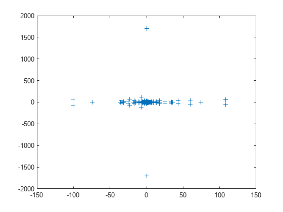
The eigenvalues are clustered along the real line (x-axis), particularly near the origin.
eigs has several options for sigma that can pick out the largest or smallest eigenvalues of varying types. Compute and plot some eigenvalues for each of the available options for sigma.
figure plot(d, '+') hold on la = eigs(A,6,'largestabs'); plot(la,'ro') sa = eigs(A,6,'smallestabs'); plot(sa,'go') hold off legend('All eigenvalues','Largest magnitude','Smallest magnitude') xlabel('Real axis') ylabel('Imaginary axis')
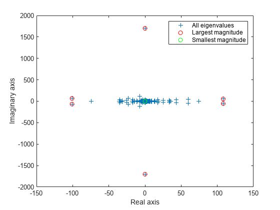
figure plot(d, '+') hold on ber = eigs(A,4,'bothendsreal'); plot(ber,'r^') bei = eigs(A,4,'bothendsimag'); plot(bei,'g^') hold off legend('All eigenvalues','Both ends real','Both ends imaginary') xlabel('Real axis') ylabel('Imaginary axis')
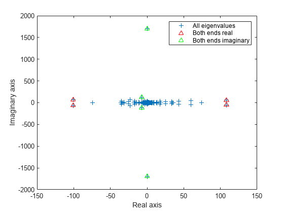
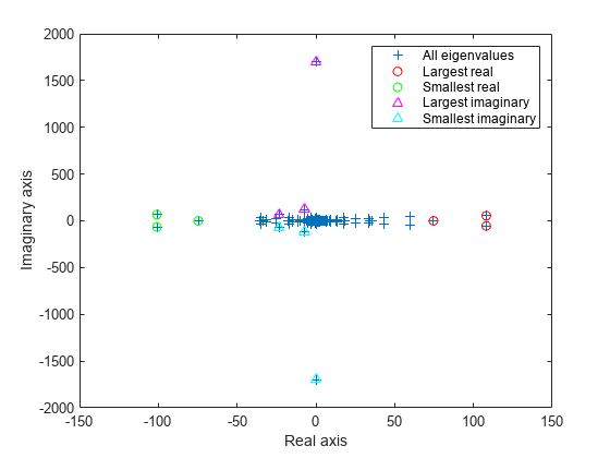
figure plot(d, '+') hold on lr = eigs(A,3,'largestreal'); plot(lr,'ro') sr = eigs(A,3,'smallestreal'); plot(sr,'go') li = eigs(A,3,'largestimag','SubspaceDimension',45); plot(li,'m^') si = eigs(A,3,'smallestimag','SubspaceDimension',45); plot(si,'c^') hold off legend('All eigenvalues','Largest real','Smallest real','Largest imaginary','Smallest imaginary') xlabel('Real axis') ylabel('Imaginary axis')
Create a symmetric positive definite sparse matrix.
A = delsq(numgrid('C', 150));
Compute the six smallest real eigenvalues using 'smallestreal', which employs a Krylov method using A.
tic d = eigs(A, 6, 'smallestreal')
d = 6×1
0.0013
0.0025
0.0033
0.0045
0.0052
0.0063
Elapsed time is 1.518482 seconds.
Compute the same eigenvalues using 'smallestabs', which employs a Krylov method using the inverse of A.
tic dsm = eigs(A, 6, 'smallestabs')
dsm = 6×1
0.0013
0.0025
0.0033
0.0045
0.0052
0.0063
Elapsed time is 0.275327 seconds.
The eigenvalues are clustered near zero. The 'smallestreal' computation struggles to converge using A since the gap between the eigenvalues is so small. Conversely, the 'smallestabs' option uses the inverse of A, and therefore the inverse of the eigenvalues of A, which have a much larger gap and are therefore easier to compute. This improved performance comes at the cost of factorizing A, which is not necessary with 'smallestreal'.
Compute eigenvalues near a numeric sigma value that is nearly equal to an eigenvalue.
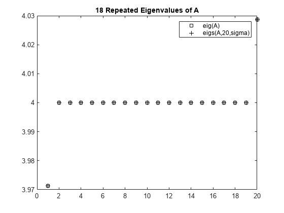
The matrix A = delsq(numgrid('C',30)) is a symmetric positive definite matrix of size 632 with eigenvalues reasonably well-distributed in the interval (0 8), but with 18 eigenvalues repeated at 4.0. To calculate some eigenvalues near 4.0, it is reasonable to try the function call eigs(A,20,4.0). However, this call computes the largest eigenvalues of the inverse of A - 4.0*I, where I is an identity matrix. Because 4.0 is an eigenvalue of A, this matrix is singular and therefore does not have an inverse. eigs fails and produces an error message. The numeric value of sigma cannot be exactly equal to an eigenvalue. Instead, you must use a value of sigma that is near but not equal to 4.0 to find those eigenvalues.
Compute all of the eigenvalues using eig, and the 20 eigenvalues closest to 4 - 1e-6 using eigs to compare results. Plot the eigenvalues calculated with each method.
A = delsq(numgrid('C',30)); sigma = 4 - 1e-6; d = eig(A); D = sort(eigs(A,20,sigma));
plot(d(307:326),'ks') hold on plot(D,'k+') hold off legend('eig(A)','eigs(A,20,sigma)') title('18 Repeated Eigenvalues of A')
Create sparse random matrices A and B that both have low densities of nonzero elements.
B = sprandn(1e3,1e3,0.001) + speye(1e3); B = B'*B; A = sprandn(1e3,1e3,0.005); A = A+A';
Find the Cholesky decomposition of matrix B, using three outputs to return the permutation vector s and test value p.
[R,p,s] = chol(B,'vector'); p
Since p is zero, B is a symmetric positive definite matrix that satisfies B(s,s) = R'*R.
Calculate the six largest magnitude eigenvalues and eigenvectors of the generalized eigenvalue problem involving A and R. Since R is the Cholesky factor of B, specify 'IsCholesky' as true. Furthermore, since B(s,s) = R'*R and thus R = chol(B(s,s)), use the permutation vector s as the value of 'CholeskyPermutation'.
[V,D,flag] = eigs(A,R,6,'largestabs','IsCholesky',true,'CholeskyPermutation',s); flag
Since flag is zero, all of the eigenvalues converged.
Input Arguments
Input matrix, specified as a square matrix. A is typically, but not always, a large and sparse matrix.
If A is symmetric, then eigs uses a specialized algorithm for that case. If A is_nearly_ symmetric, then consider using A = (A+A')/2 to make A symmetric before callingeigs. This ensures that eigs calculates real eigenvalues instead of complex ones.
Data Types: single | double
Complex Number Support: Yes
Input matrix, specified as a square matrix of the same size as A. WhenB is specified, eigs solves the generalized eigenvalue problem A*V = B*V*D.
If B is symmetric positive definite, then eigs uses a specialized algorithm for that case. If B is_nearly_ symmetric positive definite, then consider using B = (B+B')/2 to make B symmetric before calling eigs.
When A is scalar, you can specify B as an empty matrix eigs(A,[],k) to solve the standard eigenvalue problem and disambiguate between B andk.
Data Types: single | double
Complex Number Support: Yes
Number of eigenvalues to compute, specified as a positive scalar integer. Ifk is larger than size(A,2), theneigs uses the maximum valid value k = size(A,2) instead.
Example: eigs(A,2) returns the two largest eigenvalues of A.
Type of eigenvalues, specified as one of the values in the table.
| sigma | Description | sigma (R2017a and earlier) |
|---|---|---|
| scalar (real or complex, including 0) | The eigenvalues closest to the numbersigma. | No change |
| 'largestabs' (default) | Largest magnitude. | 'lm' |
| 'smallestabs' | Smallest magnitude. Same as sigma = 0. | 'sm' |
| 'largestreal' | Largest real. | 'lr', 'la' |
| 'smallestreal' | Smallest real. | 'sr', 'sa' |
| 'bothendsreal' | Both ends, with k/2 values with largest and smallest real part respectively (one more from high end if k is odd). | 'be' |
For nonsymmetric problems,sigma also can be:
| sigma | Description | sigma (R2017a and earlier) |
|---|---|---|
| 'largestimag' | Largest imaginary part. | 'li' if A is complex. |
| 'smallestimag' | Smallest imaginary part. | 'si' if A is complex. |
| 'bothendsimag' | Both ends, with k/2 values with largest and smallest imaginary part (one more from high end if k is odd). | 'li' if A is real. |
Example: eigs(A,k,1) returns the k eigenvalues closest to 1.
Example: eigs(A,k,'smallestabs') returns the k smallest magnitude eigenvalues.
Data Types: single | double | char | string
Options structure, specified as a structure containing one or more of the fields in this table.
Note
Use of the options structure to specify options is not recommended. Use name-value pairs instead.
| Option Field | Description | Name-Value Pair |
|---|---|---|
| issym | Symmetry of Afun matrix. | 'IsFunctionSymmetric' |
| tol | Convergence tolerance. | 'Tolerance' |
| maxit | Maximum number of iterations. | 'MaxIterations' |
| p | Number of Lanczos basis vectors. | 'SubspaceDimension' |
| v0 | Starting vector. | 'StartVector' |
| disp | Diagnostic information display level. | 'Display' |
| fail | Treatment of nonconverged eigenvalues in the output. | 'FailureTreatment' |
| spdB | Is B symmetric positive definite? | 'IsSymmetricDefinite' |
| cholB | Is B the Cholesky factor chol(B)? | 'IsCholesky' |
| permB | Specify the permutation vector permB if sparse B is really chol(B(permB,permB)). | 'CholeskyPermutation' |
Example: opts.issym = 1, opts.tol = 1e-10 creates a structure with values set for the fields issym and tol.
Data Types: struct
Matrix function, specified as a function handle. The function y = Afun(x) must return the proper value depending on the sigma input:
A*x— Ifsigmais unspecified or any text option other than'smallestabs'.A\x— Ifsigmais0or'smallestabs'.(A-sigma*I)\x— Ifsigmais a nonzero scalar (for standard eigenvalue problem).(A-sigma*B)\x— Ifsigmais a nonzero scalar (for generalized eigenvalue problem).
For example, the following Afun works when calling eigs with sigma = 'smallestabs':
[L,U,p] = lu(A,'vector'); Afun = @(x) U(L(x(p))); d = eigs(Afun,100,6,'smallestabs')
For a generalized eigenvalue problem, add matrix B as follows (B cannot be represented by a function handle):
d = eigs(Afun,100,B,6,'smallestabs')
A is assumed to be nonsymmetric unless'IsFunctionSymmetric' (oropts.issym) specifies otherwise. Setting'IsFunctionSymmetric' to true ensures that eigs calculates real eigenvalues instead of complex ones.
For information on how to provide additional parameters to theAfun function, see Parameterizing Functions.
Tip
Call eigs with the 'Display' option turned on to see what output is expected fromAfun.
Size of square matrix A that is represented byAfun, specified as a positive scalar integer.
Name-Value Arguments
Specify optional pairs of arguments asName1=Value1,...,NameN=ValueN, where Name is the argument name and Value is the corresponding value. Name-value arguments must appear after other arguments, but the order of the pairs does not matter.
Before R2021a, use commas to separate each name and value, and enclose Name in quotes.
Example: d = eigs(A,k,sigma,'Tolerance',1e-10,'MaxIterations',100) loosens the convergence tolerance and uses fewer iterations.
General Options
Convergence tolerance, specified as the comma-separated pair consisting of 'Tolerance' and a positive real numeric scalar.
Example: s = eigs(A,k,sigma,'Tolerance',1e-3)
Maximum number of algorithm iterations, specified as the comma-separated pair consisting of 'MaxIterations' and a positive integer.
Example: d = eigs(A,k,sigma,'MaxIterations',350)
Maximum size of Krylov subspace, specified as the comma-separated pair consisting of 'SubspaceDimension' and a nonnegative integer. The 'SubspaceDimension' value must be greater than or equal to k + 1 for real symmetric problems, and k + 2 otherwise, wherek is the number of eigenvalues.
The recommended value is p >= 2*k, or for real nonsymmetric problems, p >= 2*k+1. If you do not specify a 'SubspaceDimension' value, then the default algorithm uses at least 20 Lanczos vectors.
For problems where eigs fails to converge, increasing the value of 'SubspaceDimension' can improve the convergence behavior. However, increasing the value too much can cause memory issues.
Example: d = eigs(A,k,sigma,'SubspaceDimension',25)
Initial starting vector, specified as the comma-separated pair consisting of 'StartVector' and a numeric vector.
The primary reason to specify a different random starting vector is when you want to control the random number stream used to generate the vector.
Note
eigs selects the starting vectors in a reproducible manner using a private random number stream. Changing the random number seed does not affect the starting vector.
Example: d = eigs(A,k,sigma,'StartVector',randn(m,1)) uses a random starting vector that draws values from the global random number stream.
Data Types: single | double
Treatment of nonconverged eigenvalues, specified as the comma-separated pair consisting of 'FailureTreatment' and one of the options: 'replacenan','keep', or 'drop'.
The value of 'FailureTreatment' determines howeigs displays nonconverged eigenvalues in the output.
| Option | Affect on output |
|---|---|
| 'replacenan' | Replace nonconverged eigenvalues withNaN values. |
| 'keep' | Include nonconverged eigenvalues in the output. |
| 'drop' | Remove nonconverged eigenvalues from the output. This option can result in eigs returning fewer eigenvalues than requested. |
Example: d = eigs(A,k,sigma,'FailureTreatment','drop') removes nonconverged eigenvalues from the output.
Data Types: char | string
Toggle for diagnostic information display, specified as the comma-separated pair consisting of 'Display' and a numeric or logical 1 (true) or0 (false). Specify a value oftrue or 1 to turn on the display of diagnostic information during the calculation.
Options for Afun
Symmetry of Afun matrix, specified as the comma-separated pair consisting of'IsFunctionSymmetric' and a numeric or logical1 (true) or0 (false).
This option specifies whether the matrix that Afun applies to its input vector is symmetric. Specify a value oftrue or 1 to indicate thateigs should use a specialized algorithm for the symmetric matrix and return real eigenvalues.
Options for generalized eigenvalue problem A*V = B*V*D
Cholesky decomposition toggle for B, specified as the comma-separated pair consisting of 'IsCholesky' and a numeric or logical 1 (true) or 0 (false).
This option specifies whether the input for matrixB in the call eigs(A,B,___) is actually the Cholesky factor R produced by R = chol(B).
Note
Do not use this option if sigma is'smallestabs' or a numeric scalar.
Cholesky permutation vector, specified as the comma-separated pair consisting of 'CholeskyPermutation' and a numeric vector. Specify the permutation vector permB if sparse matrix B is reordered before factorization according to chol(B(permB,permB)).
You also can use the three-output syntax of chol for sparse matrices to directly obtain permB with[R,p,permB] = chol(B,'vector').
Note
Do not use this option if sigma is'smallestabs' or a numeric scalar.
Symmetric-positive-definiteness toggle for B, specified as the comma-separated pair consisting of'IsSymmetricDefinite' and a numeric or logical1 (true) or0 (false). Specifytrue or 1 when you know thatB is symmetric positive definite, that is, it is a symmetric matrix with strictly positive eigenvalues.
If B is symmetric positive semi-definite (some eigenvalues are zero), then specifying'IsSymmetricDefinite' as true or 1 forces eigs to use the same specialized algorithm that it uses when B is symmetric positive definite.
Note
To use this option, the value of sigma must be numeric or 'smallestabs'.
Output Arguments
Eigenvalues, returned as a column vector. d is sorted differently depending on the value of sigma.
| Value of sigma | Output sorting |
|---|---|
| 'largestabs' | Descending order by magnitude |
| 'largestreal' | Descending order by real part |
| 'largestimag' | Descending order by imaginary part |
| 'smallestabs' | Ascending order by magnitude |
| 'smallestreal' 'bothendsreal' | Ascending order by real part |
| 'smallestimag' | Ascending order by imaginary part |
| 'bothendsimag' | Descending order by absolute value of imaginary part |
Eigenvectors, returned as a matrix. The columns in V correspond to the eigenvalues along the diagonal of D. The form and normalization of V depends on the combination of input arguments:
[V,D] = eigs(A)returns matrixV, whose columns are the right eigenvectors ofAsuch thatA*V = V*D. The eigenvectors inVare normalized so that the 2-norm of each is 1.
IfAis symmetric, then the eigenvectors,V, are orthonormal.[V,D] = eigs(A,B)returnsVas a matrix whose columns are the generalized right eigenvectors that satisfyA*V = B*V*D. The 2-norm of each eigenvector is not necessarily 1.
IfBis symmetric positive definite, then the eigenvectors inVare normalized so that theB-norm of each is 1. IfAis also symmetric, then the eigenvectors areB-orthonormal.
Different machines, releases of MATLAB®, or parameters (such as the starting vector and subspace dimension) can produce different eigenvectors that are still numerically accurate:
- For real eigenvectors, the sign of the eigenvectors can change.
- For complex eigenvectors, the eigenvectors can be multiplied by any complex number of magnitude 1.
- For a multiple eigenvalue, its eigenvectors can be recombined through linear combinations. For example, if A x =λ x and A y =λ y, then A(x+y) =λ(x+y), so x+y also is an eigenvector of_A_.
Eigenvalue matrix, returned as a diagonal matrix with the eigenvalues on the main diagonal.
Convergence flag, returned as 0 or 1. A value of0 indicates that all the eigenvalues converged. Otherwise, not all of the eigenvalues converged.
Use of this convergence flag output suppresses warnings about failed convergence.
Tips
eigsgenerates the default starting vector using a private random number stream to ensure reproducibility across runs. Setting the random number generator state using rng before callingeigsdoes not affect the output.- Using
eigsis not the most efficient way to find a few eigenvalues of small, dense matrices. For such problems, it might be quicker to useeig(full(A)). For example, finding three eigenvalues in a 500-by-500 matrix is a relatively small problem that is easily handled witheig. - If
eigsfails to converge for a given matrix, increase the number of Lanczos basis vectors by increasing the value of'SubspaceDimension'. As secondary options, adjusting the maximum number of iterations,'MaxIterations', and the convergence tolerance,'Tolerance', also can help with convergence behavior.
References
[1] Stewart, G.W. "A Krylov-Schur Algorithm for Large Eigenproblems." SIAM Journal of Matrix Analysis and Applications. Vol. 23, Issue 3, 2001, pp. 601–614.
[2] Lehoucq, R.B., D.C. Sorenson, and C. Yang. ARPACK Users' Guide. Philadelphia, PA: SIAM, 1998.
Extended Capabilities
Version History
Introduced before R2006a
You can specify these arguments as single precision:
A,B— Input matricessigma— Type of eigenvaluesStartVector— Initial starting vector
If you specify A, B, orStartVector as single precision, the function computes in single precision and returns outputs of type single.
If you specify only the matrix function Afun and the matrix size n as inputs, the outputs of eigs are of the same precision as the output of Afun. If you also specify either B or StartVector assingle, then the output of Afun must also besingle.
- Changes to sorting order of output
eigsnow sorts the output according to the value ofsigma. For example, the commandeigs(A,k,'largestabs')produceskeigenvalues sorted in descending order by magnitude.
Previously, the sorting order of the output produced byeigswas not guaranteed. - Reproducibility
Callingeigsmultiple times in succession now produces the same result. Set'StartVector'to a random vector to change this behavior. - Display
A display value of2no longer returns timing information. Instead,eigstreats a value of2the same as a value of1. Also, the messages shown by the'Display'option have changed. The new messages show the residual in each iteration, instead of the Ritz values.