Histogram2 - Bivariate histogram plot - MATLAB (original) (raw)

Description
Bivariate histograms are a type of bar plot for numeric data that group the data into 2-D bins. After you create a Histogram2 object, you can modify aspects of the histogram by changing its property values. This is particularly useful for quickly modifying the properties of the bins or changing the display.
Creation
Syntax
Description
histogram2([X,Y](#buvhqen-XY)) creates a bivariate histogram plot of X and Y. The histogram2 function uses an automatic binning algorithm that returns bins with a uniform area, chosen to cover the range of elements in X and Y and reveal the underlying shape of the distribution. histogram2 displays the bins as 3-D rectangular bars such that the height of each bar indicates the number of elements in the bin.
histogram2([X,Y](#buvhqen-XY),[nbins](#mw%5F484c4be6-77ab-4db9-83ca-8f136a263472)) specifies the number of bins to use in each dimension.
histogram2([X,Y](#buvhqen-XY),[Xedges](#mw%5F86091e22-4387-4d73-8b5a-4f2a66dccedf),[Yedges](#mw%5F9fdd3158-3ef3-4551-8e9f-fd947ca692ca)) sorts X and Y into bins with the bin edges for each dimension specified in vectors.
histogram2('XBinEdges',[Xedges](#mw%5F86091e22-4387-4d73-8b5a-4f2a66dccedf),'YBinEdges',[Yedges](#mw%5F9fdd3158-3ef3-4551-8e9f-fd947ca692ca),'BinCounts',[counts](#buvhqen-counts)) plots the specified bin counts and does not do any data binning.
histogram2(___,[Name,Value](#namevaluepairarguments)) specifies additional parameters using one or more name-value arguments for any of the previous syntaxes. For example, specifyNormalization to use a different type of normalization. For a list of properties, see Histogram2 Properties.
histogram2([ax](#buvhqen-ax),___) plots into the specified axes instead of into the current axes (gca). ax can precede any of the input argument combinations in the previous syntaxes.
[h](#buvhqen-h) = histogram2(___) returns a Histogram2 object. Use this to inspect and adjust properties of the bivariate histogram. For a list of properties, seeHistogram2 Properties.
Input Arguments
Data to distribute among bins, specified as separate arguments of vectors, matrices, or multidimensional arrays. X andY must be the same size.histogram2 treats matrix or multidimensional array data as single column vectors, X(:) andY(:), and plots a single histogram.
Corresponding elements in X andY specify the x and_y_ coordinates of 2-D data points,[X(k),Y(k)]. The data types ofX and Y can be different, buthistogram2 concatenates these inputs into a single N-by-2 matrix of the dominant data type.
histogram2 ignores all NaN values. Similarly, histogram2 ignoresInf and -Inf values, unless the bin edges explicitly specify Inf or-Inf as a bin edge. AlthoughNaN, Inf, and-Inf values are typically not plotted, they are still included in normalization calculations that include the total number of data elements, such as'probability'.
Note
If X or Y contain integers of type int64 or uint64 that are larger than flintmax, then it is recommended that you explicitly specify the histogram bin edges.histogram2 automatically bins the input data using double precision, which lacks integer precision for numbers greater than flintmax.
Data Types: single | double | int8 | int16 | int32 | int64 | uint8 | uint16 | uint32 | uint64 | logical
Number of bins in each dimension, specified as a positive integer scalar or two-element vector of positive integers.
- If
nbinsis a scalar, thenhistogram2uses that many bins in each dimension. - If
nbinsis a vector, then the first element gives the number of bins in the_x_-dimension, and the second element gives the number of bins in the _y_-dimension.
If you do not specify nbins, thenhistogram2 automatically calculates how many bins to use based on the values inX and Y.
If you specify nbins withBinMethod or BinWidth,histogram2 only honors the last parameter.
Example: histogram2(X,Y,20) uses 20 bins in each dimension.
Example: histogram2(X,Y,[10 20]) uses 10 bins in thex-dimension and 20 bins in they-dimension.
Bin edges in _x_-dimension, specified as a vector. The first element specifies the leading edge of the first bin in the_x_-dimension. The last element specifies the trailing edge of the last bin in the _x_-dimension. The trailing edge is only included for the last bin.
- If you specify
XedgesandYedgeswithBinMethod,BinWidth, orNumBins,histogram2only honors the bin edges and the bin edges must be specified last. - If you specify
XedgeswithXBinLimits,histogram2only honors theXedgesand theXedgesmust be specified last.
Bin edges in _y_-dimension, specified as a vector. The first element specifies the leading edge of the first bin in the_y_-dimension. The last element specifies the trailing edge of the last bin in the _y_-dimension. The trailing edge is only included for the last bin.
- If you specify
YedgesandXedgeswithBinMethod,BinWidth, orNumBins,histogram2only honors the bin edges and the bin edges must be specified last. - If you specify
YedgeswithYBinLimits,histogram2only honors theYedgesand theYedgesmust be specified last.
Bin counts, specified as a matrix. Use this input to pass bin counts to histogram2 when the bin counts calculation is performed separately and you do not want histogram2 to do any data binning.
counts must be a matrix of size[length(XBinEdges)-1 length(YBinEdges)-1] so that it specifies a bin count for each bin.
Example: histogram2('XBinEdges',-1:1,'YBinEdges',-2:2,'BinCounts',[1 2 3 4; 5 6 7 8])
Axes object. If you do not specify an axes, then thehistogram2 function uses the current axes (gca).
Name-Value Arguments
Specify optional pairs of arguments asName1=Value1,...,NameN=ValueN, where Name is the argument name and Value is the corresponding value. Name-value arguments must appear after other arguments, but the order of the pairs does not matter.
Example: histogram2(X,Y,BinWidth=[5 10])
Before R2021a, use commas to separate each name and value, and enclose Name in quotes.
Example: histogram2(X,Y,'BinWidth',[5 10])
Bins
Bin limits in _x_-dimension, specified as a two-element vector,[xbmin,xbmax]. The first element indicates the first bin edge in the _x_-dimension. The second element indicates the last bin edge in the _x_-dimension.
This option only bins data that falls within the bin limits inclusively,X>=xbmin & X<=xbmax.
Selection mode for bin limits in x-dimension, specified as'auto' or 'manual'. The default value is'auto', so that the bin limits automatically adjust to the data along the x-axis.
If you explicitly specify either XBinLimits orXBinEdges, then XBinLimitsMode is set automatically to 'manual'. In that case, specifyXBinLimitsMode as 'auto' to rescale the bin limits to the data.
Bin limits in _y_-dimension, specified as a two-element vector,[ybmin,ybmax]. The first element indicates the first bin edge in the _y_-dimension. The second element indicates the last bin edge in the _y_-dimension.
This option only bins data that falls within the bin limits inclusively,Y>=ybmin & Y<=ybmax.
Selection mode for bin limits in _y_-dimension, specified as'auto' or 'manual'. The default value is'auto', so that the bin limits automatically adjust to the data along the _y_-axis.
If you explicitly specify either YBinLimits orYBinEdges, then YBinLimitsMode is set automatically to 'manual'. In that case, specifyYBinLimitsMode as 'auto' to rescale the bin limits to the data.
Toggle display of empty bins, specified as either'off' or 'on'. The default value is 'off'.
Example: histogram2(X,Y,'ShowEmptyBins','on') turns on the display of empty bins.
Data
Color and Styling
Histogram display style, specified as either 'bar3' or'tile'.
'bar3'— Display the histogram using 3-D bars.'tile'— Display the histogram as a rectangular array of tiles with colors indicating the bin values.
Example: histogram2(X,Y,'DisplayStyle','tile') plots the histogram as a rectangular array of tiles.
Lighting effect on histogram bars, specified as one of these values.
| Value | Description |
|---|---|
| 'lit' | Histogram bars display a pseudo-lighting effect, where the sides of the bars use darker colors relative to the tops. The bars are unaffected by other light sources in the axes. This is the default value when DisplayStyle is'bar3'. |
| 'flat' | Histogram bars are not lit automatically. In the presence of other light objects, the lighting effect is uniform across the bar faces. |
| 'none' | Histogram bars are not lit automatically, and lights do not affect the histogram bars. FaceLighting can only be'none' when DisplayStyle is 'tile'. |
Example: histogram2(X,Y,'FaceLighting','none') turns off the lighting of the histogram bars.
Data Types: single | double | int8 | int16 | int32 | int64 | uint8 | uint16 | uint32 | uint64
Output Arguments
Properties
Object Functions
Examples
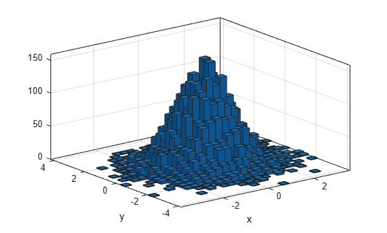
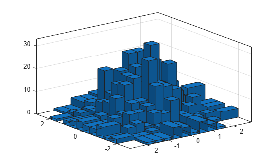
Generate 10,000 pairs of random numbers and create a bivariate histogram. The histogram2 function automatically chooses an appropriate number of bins to cover the range of values in x and y and show the shape of the underlying distribution.
x = randn(10000,1); y = randn(10000,1); h = histogram2(x,y)
h = Histogram2 with properties:
         Data: [10000×2 double]
       Values: [25×28 double]
      NumBins: [25 28]
    XBinEdges: [-3.9000 -3.6000 -3.3000 -3 -2.7000 -2.4000 -2.1000 -1.8000 -1.5000 -1.2000 -0.9000 -0.6000 -0.3000 0 0.3000 0.6000 0.9000 1.2000 1.5000 1.8000 2.1000 2.4000 2.7000 3.0000 3.3000 3.6000]
    YBinEdges: [-4.2000 -3.9000 -3.6000 -3.3000 -3.0000 -2.7000 -2.4000 -2.1000 -1.8000 -1.5000 -1.2000 -0.9000 -0.6000 -0.3000 0 0.3000 0.6000 0.9000 1.2000 1.5000 1.8000 2.1000 2.4000 2.7000 3 3.3000 3.6000 3.9000 4.2000]
     BinWidth: [0.3000 0.3000]
Normalization: 'count'
    FaceColor: 'auto'
    EdgeColor: [0.1294 0.1294 0.1294]
Show all properties
When you specify an output argument to the histogram2 function, it returns a histogram2 object. You can use this object to inspect the properties of the histogram, such as the number of bins or the width of the bins.
Find the number of histogram bins in each dimension.
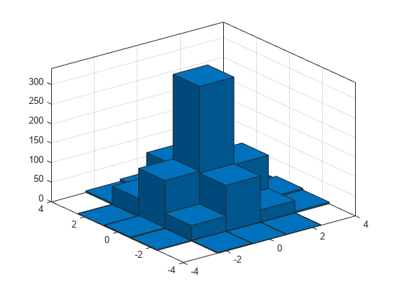
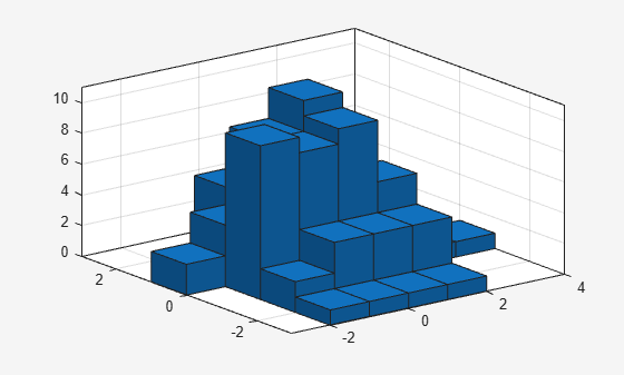
Plot a bivariate histogram of 1,000 pairs of random numbers sorted into 25 equally spaced bins, using 5 bins in each dimension.
x = randn(1000,1); y = randn(1000,1); nbins = 5; h = histogram2(x,y,nbins)
h = Histogram2 with properties:
         Data: [1000×2 double]
       Values: [5×5 double]
      NumBins: [5 5]
    XBinEdges: [-4 -2.4000 -0.8000 0.8000 2.4000 4]
    YBinEdges: [-4 -2.4000 -0.8000 0.8000 2.4000 4]
     BinWidth: [1.6000 1.6000]
Normalization: 'count'
    FaceColor: 'auto'
    EdgeColor: [0.1294 0.1294 0.1294]
Show all properties
Find the resulting bin counts.
counts = 5×5
0 2 3 1 0
2 40 124 47 4
1 119 341 109 10
1 32 117 33 1
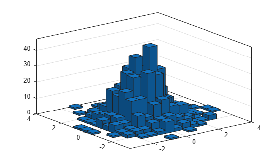
0 4 8 1 0Generate 1,000 pairs of random numbers and create a bivariate histogram.
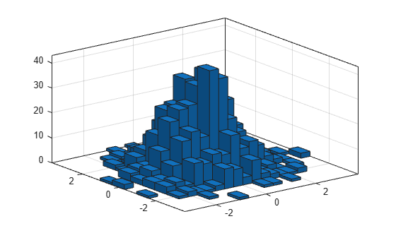
x = randn(1000,1); y = randn(1000,1); h = histogram2(x,y)
h = Histogram2 with properties:
         Data: [1000×2 double]
       Values: [15×15 double]
      NumBins: [15 15]
    XBinEdges: [-3.5000 -3 -2.5000 -2 -1.5000 -1 -0.5000 0 0.5000 1 1.5000 2 2.5000 3 3.5000 4]
    YBinEdges: [-3.5000 -3 -2.5000 -2 -1.5000 -1 -0.5000 0 0.5000 1 1.5000 2 2.5000 3 3.5000 4]
     BinWidth: [0.5000 0.5000]
Normalization: 'count'
    FaceColor: 'auto'
    EdgeColor: [0.1294 0.1294 0.1294]
Show all properties
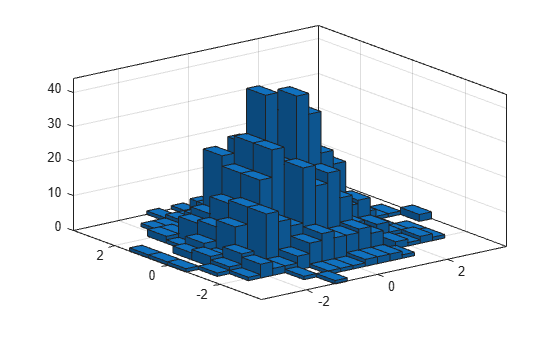
Use the morebins function to coarsely adjust the number of bins in the x dimension.
nbins = morebins(h,'x'); nbins = morebins(h,'x')
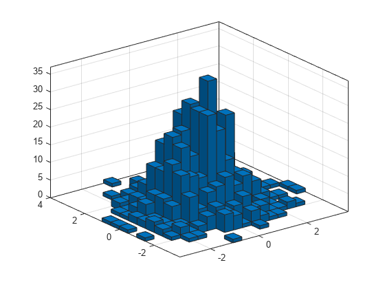
Use the fewerbins function to adjust the number of bins in the y dimension.
nbins = fewerbins(h,'y'); nbins = fewerbins(h,'y')
Adjust the number of bins at a fine grain level by explicitly setting the number of bins.
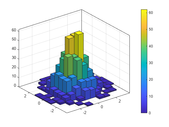
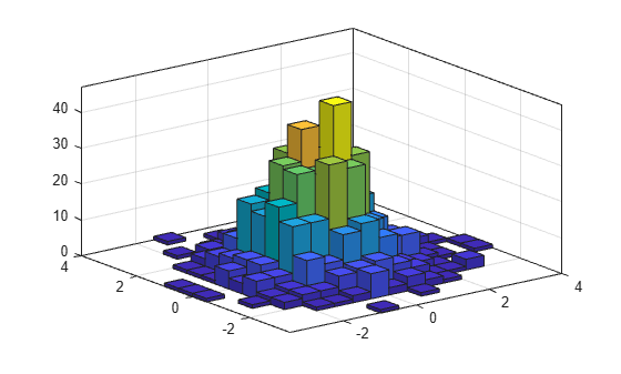
Create a bivariate histogram using 1,000 normally distributed random numbers with 12 bins in each dimension. Specify FaceColor as 'flat' to color the histogram bars by height.
h = histogram2(randn(1000,1),randn(1000,1),[12 12],'FaceColor','flat'); colorbar
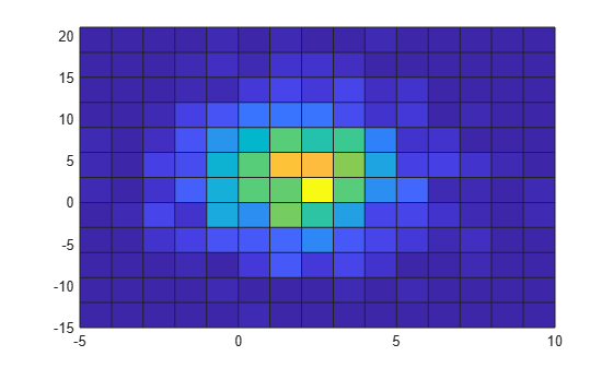
Generate random data and plot a bivariate tiled histogram. Display the empty bins by specifying ShowEmptyBins as 'on'.
x = 2randn(1000,1)+2; y = 5randn(1000,1)+3; h = histogram2(x,y,'DisplayStyle','tile','ShowEmptyBins','on');
Generate 1,000 pairs of random numbers and create a bivariate histogram. Specify the bin edges using two vectors, with infinitely wide bins on the boundary of the histogram to capture all outliers that do not satisfy |x|<2.
x = randn(1000,1); y = randn(1000,1); Xedges = [-Inf -2:0.4:2 Inf]; Yedges = [-Inf -2:0.4:2 Inf]; h = histogram2(x,y,Xedges,Yedges)
h = Histogram2 with properties:
         Data: [1000×2 double]
       Values: [12×12 double]
      NumBins: [12 12]
    XBinEdges: [-Inf -2 -1.6000 -1.2000 -0.8000 -0.4000 0 0.4000 0.8000 1.2000 1.6000 2 Inf]
    YBinEdges: [-Inf -2 -1.6000 -1.2000 -0.8000 -0.4000 0 0.4000 0.8000 1.2000 1.6000 2 Inf]
     BinWidth: 'nonuniform'
Normalization: 'count'
    FaceColor: 'auto'
    EdgeColor: [0.1294 0.1294 0.1294]
Show all properties
When the bin edges are infinite, histogram2 displays each outlier bin (along the boundary of the histogram) as being double the width of the bin next to it.
Specify the Normalization property as 'countdensity' to remove the bins containing the outliers. Now the volume of each bin represents the frequency of observations in that interval.
h.Normalization = 'countdensity';

Generate 1,000 pairs of random numbers and create a bivariate histogram using the 'probability' normalization.
x = randn(1000,1); y = randn(1000,1); h = histogram2(x,y,'Normalization','probability')

h = Histogram2 with properties:
         Data: [1000×2 double]
       Values: [15×15 double]
      NumBins: [15 15]
    XBinEdges: [-3.5000 -3 -2.5000 -2 -1.5000 -1 -0.5000 0 0.5000 1 1.5000 2 2.5000 3 3.5000 4]
    YBinEdges: [-3.5000 -3 -2.5000 -2 -1.5000 -1 -0.5000 0 0.5000 1 1.5000 2 2.5000 3 3.5000 4]
     BinWidth: [0.5000 0.5000]
Normalization: 'probability'
    FaceColor: 'auto'
    EdgeColor: [0.1294 0.1294 0.1294]
Show all properties
Compute the total sum of the bar heights. With this normalization, the height of each bar is equal to the probability of selecting an observation within that bin interval, and the heights of all of the bars sum to 1.
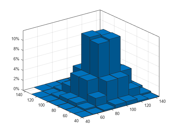
Generate 100,000 normally distributed random vectors. Use a standard deviation of 15 and means of 100 and 85.
x = [100 85] + 15*randn(1e5,2);
Plot a histogram of the random vectors. Scale and label the _z_-axis as percentages.
edges = 40:15:145; histogram2(x(:,1),x(:,2),edges,edges,Normalization="percentage") ztickformat("percentage")
Generate 1,000 pairs of random numbers and create a bivariate histogram. Return the histogram object to adjust the properties of the histogram without recreating the entire plot.
x = randn(1000,1); y = randn(1000,1); h = histogram2(x,y)

h = Histogram2 with properties:
         Data: [1000×2 double]
       Values: [15×15 double]
      NumBins: [15 15]
    XBinEdges: [-3.5000 -3 -2.5000 -2 -1.5000 -1 -0.5000 0 0.5000 1 1.5000 2 2.5000 3 3.5000 4]
    YBinEdges: [-3.5000 -3 -2.5000 -2 -1.5000 -1 -0.5000 0 0.5000 1 1.5000 2 2.5000 3 3.5000 4]
     BinWidth: [0.5000 0.5000]
Normalization: 'count'
    FaceColor: 'auto'
    EdgeColor: [0.1294 0.1294 0.1294]
Show all properties
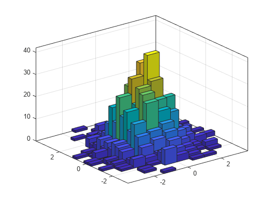
Color the histogram bars by height.
Change the number of bins in each direction.
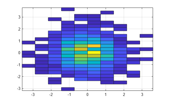
Display the histogram as a tile plot.
h.DisplayStyle = 'tile'; view(2)
Use the savefig function to save a histogram2 figure.
histogram2(randn(100,1),randn(100,1)); savefig('histogram2.fig'); close gcf
Use openfig to load the histogram figure back into MATLAB®. openfig also returns a handle to the figure, h.
h = openfig('histogram2.fig');
Use the findobj function to locate the correct object handle from the figure handle. This allows you to continue manipulating the original histogram object used to generate the figure.
y = findobj(h,'type','histogram2')
y = Histogram2 with properties:
         Data: [100×2 double]
       Values: [7×6 double]
      NumBins: [7 6]
    XBinEdges: [-3 -2 -1 0 1 2 3 4]
    YBinEdges: [-3 -2 -1 0 1 2 3]
     BinWidth: [1 1]
Normalization: 'count'
    FaceColor: 'auto'
    EdgeColor: [0.1294 0.1294 0.1294]
Show all properties
Tips
- Histogram plots created using
histogram2have a context menu in plot edit mode that enables interactive manipulations in the figure window. For example, you can use the context menu to interactively change the number of bins, align multiple histograms, or change the display order.
Extended Capabilities
This function supports tall arrays with the limitations:
- Some input options are not supported. The allowed options are:
'BinWidth''XBinLimits''YBinLimits''Normalization''DisplayStyle''BinMethod'— The'auto'and'scott'bin methods are the same. The'fd'bin method is not supported.'EdgeAlpha''EdgeColor''FaceAlpha''FaceColor''LineStyle''LineWidth''Orientation'
- Additionally, there is a cap on the maximum number of bars. The default maximum is 100.
- The
morebinsandfewerbinsmethods are not supported. - Editing properties of the histogram object that require recomputing the bins is not supported.
For more information, see Tall Arrays for Out-of-Memory Data.
Version History
Introduced in R2015b
You can create histograms with percentages on the vertical axis by setting theNormalization name-value argument to'percentage'.