ScatterHistogramChart - Control scatter histogram chart appearance and behavior - MATLAB (original) (raw)
ScatterHistogramChart Properties
Control scatter histogram chart appearance and behavior
ScatterHistogramChart properties control the appearance and behavior of a ScatterHistogramChart object. By changing property values, you can modify certain aspects of the chart display. For example, you can add a title:
s = scatterhistogram(rand(10,1),rand(10,1)); s.Title = 'My Title';
Labels
Label for the _x_-axis, specified as a character vector, string array, cell array of character vectors, or categorical array. Use '' for no label.
To create a multiline label, specify a string array or cell array of character vectors. Each element in the array corresponds to a line of text.
If you specify the label as a categorical array, MATLAB uses the values in the array, not the categories.
Example: s = scatterhistogram(__,'XLabel','My Label')
Example: s.XLabel = 'My Label'
Example: s.XLabel = {'My','Label'}
Label for the _y_-axis, specified as a character vector, string array, cell array of character vectors, or categorical array. Use '' for no label.
To create a multiline label, specify a string array or cell array of character vectors. Each element in the array corresponds to a line of text.
If you specify the label as a categorical array, MATLAB uses the values in the array, not the categories.
Example: s = scatterhistogram(__,'YLabel','My Label')
Example: s.YLabel = 'My Label'
Example: s.YLabel = {'My','Label'}
Legend title, specified as a character vector, string array, cell array of character vectors, or categorical array. Use '' for no title.
To create a multiline title, specify a string array or cell array of character vectors. Each element in the array corresponds to a line of text.
If you specify the title as a categorical array, MATLAB uses the values in the array, not the categories.
Example: s = scatterhistogram(__,'LegendTitle','My Title Text')
Example: s.LegendTitle = 'My Title Text'
Example: s.LegendTitle = {'My','Title'}
Histograms
Histogram bin widths, specified as a positive scalar, 2-by-1 positive vector, or 2-by-n positive matrix, where n is the number of groups in GroupData.
| Specified Value | Description |
|---|---|
| scalar | The value is the bin width for the x and_y_ histograms. |
| 2-by-1 vector | The first value is the bin width for the x data, and the second value is the bin width for the y data. |
| 2-by-n matrix | The (1,j) value is the bin width for the histogram of the x data that is in the jth group. Similarly, the (2,j) value is the bin width for the histogram of the y data that is in the jth group. |
scatterhistogram uses the 'BinMethod','auto' name-value pair argument of histogram to determine the defaultNumBins and BinWidths values. TheBinWidths values for categorical data are always0. When HistogramDisplayStyle is"smooth", BinWidths is the bandwidth for the kernel density estimator kde.
If you set BinWidths, thenscatterhistogram ignores the NumBins value.
Example: s = scatterhistogram(__,'BinWidths',0.5)
Example: s.BinWidths = [1.5; 2]
Direction of the x data histograms, specified as'up' or 'down'. If theXHistogramDirection value is 'up', then the_x_ data histograms have bars directed upwards. If theXHistogramDirection value is 'down', then the_x_ data histograms have bars directed downwards.
Example: s = scatterhistogram(__,'XHistogramDirection','down')
Example: s.XHistogramDirection = 'down'
Direction of the y data histograms, specified as'right' or 'left'. If theYHistogramDirection value is 'right', then the_y_ data histograms have bars directed rightwards. If theYHistogramDirection value is 'left', then the_y_ data histograms have bars directed leftwards.
Example: s = scatterhistogram(__,'YHistogramDirection','left')
Example: s.YHistogramDirection = 'left'
Histogram line style, specified in one of these forms:
- Character vector designating one line style
- String array or cell array of character vectors designating one or more line styles
Choose among these line style options.
| Line Style | Description | Resulting Line |
|---|---|---|
| "-" | Solid line |  |
| "--" | Dashed line |  |
| ":" | Dotted line |  |
| "-." | Dash-dotted line |  |
| "none" | No line | No line |
When the total number of groups exceeds the number of specified line styles,scatterhistogram cycles through the specified line styles.
Example: s = scatterhistogram(__,'LineStyle',':')
Example: s.LineStyle = {':','-','-.'}
Color and Font
Group color, specified in one of these forms:
- Character vector designating a color name.
- String array or cell array of character vectors designating one or more color names.
- Three-column matrix of RGB values in the range [0,1]. The three columns represent the R value, G value, and B value, respectively.
Choose among these predefined colors and their equivalent RGB triplets.
| Option | Description | Equivalent RGB Triplet |
|---|---|---|
| 'red' or 'r' | Red | [1 0 0] |
| 'green' or 'g' | Green | [0 1 0] |
| 'blue' or 'b' | Blue | [0 0 1] |
| 'yellow' or 'y' | Yellow | [1 1 0] |
| 'magenta' or 'm' | Magenta | [1 0 1] |
| 'cyan' or 'c' | Cyan | [0 1 1] |
| 'white' or 'w' | White | [1 1 1] |
| 'black' or 'k' | Black | [0 0 0] |
By default, scatterhistogram assigns a maximum of seven unique group colors. When the total number of groups exceeds the number of specified colors,scatterhistogram cycles through the specified colors.
Example: s = scatterhistogram(__,'Color',{'blue','green',red'})
Example: s.Color = [0 0 1; 0 0.5 0.5; 0.5 0.5 0.5]
Font name, specified as a system-supported font name. The same font is used for the title, axis labels, legend title, and group names. The default font depends on the specific operating system and locale.
Example: s = scatterhistogram(__,'FontName','Cambria')
Example: s.FontName = 'Cambria'
Font size, specified as a scalar value. FontSize is the same for the title, axis labels, legend title, and group names. The default font size depends on the specific operating system and locale.
As you adjust the size of plot elements, the software automatically updates the font size. However, changing the FontSize property disables this automatic resizing.
Example: s = scatterhistogram(__,'FontSize',12)
Example: s.FontSize = 12
Markers
Marker size for each scatter plot group, specified as a nonnegative scalar or nonnegative vector, with values measured in points. By default,scatterhistogram assigns 36 as the marker size for each group in the scatter plot. When the total number of groups exceeds the number of specified values, scatterhistogram cycles through the specified values.
Example: s = scatterhistogram(__,'MarkerSize',30)
Example: s.MarkerSize = 40
State of marker face fill, specified as 'on' or'off'. If MarkerFilled is set to'on', then scatterhistogram fills the interior of the markers in the scatter plot. If MarkerFilled is set to'off', then scatterhistogram leaves the interior of the scatter plot markers empty.
Example: s = scatterhistogram(__,'MarkerFilled','off')
Example: s.MarkerFilled = 'off'
Marker transparency for each scatter plot group, specified as a numeric scalar or numeric vector with values between 0 and 1. Values closer to 0 specify more transparent markers, and values closer to 1 specify more opaque markers. By default,scatterhistogram assigns a MarkerAlpha value of 1 to all markers in the scatter plot.
Example: s = scatterhistogram(__,'MarkerAlpha',0.75)
Example: s.MarkerAlpha = [0.2 0.7 0.4]
Layout
Ratio of the scatter plot length to the overall chart length, specified as a numeric scalar between 0 and 1. The ScatterPlotProportion value applies to both x and y axes.
Example: s = scatterhistogram(__,'ScatterPlotProportion',0.7)
Example: s.ScatterPlotProportion = 0.6
Position
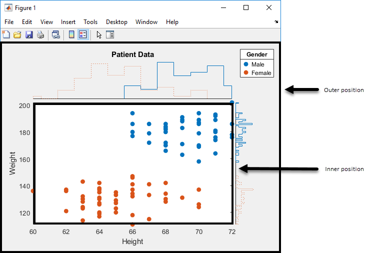
Position property to hold constant when adding, removing, or changing decorations, specified as one of the following values:
'outerposition'— TheOuterPositionproperty remains constant when you add, remove, or change decorations such as a title or an axis label. If any positional adjustments are needed, MATLAB adjusts theInnerPositionproperty.'innerposition'— TheInnerPositionproperty remains constant when you add, remove, or change decorations such as a title or an axis label. If any positional adjustments are needed, MATLAB adjusts theOuterPositionproperty.
This figure shows the innerposition andouterposition definitions forScatterHistogramChart.
Example: s.PositionConstraint = 'outerposition'
Note
Setting this property has no effect when the parent container is aTiledChartLayout object.
Inner size and position of the chart within the parent container (typically a figure, panel, or tab), specified as a four-element numeric vector of the form[left bottom width height]. The inner position includes only the scatter plot.
- The
leftandbottomelements define the distance from the lower left corner of the container to the lower left corner of the scatter plot. - The
widthandheightelements are the dimensions of the scatter plot.
For an illustration, see PositionConstraint.
Note
Setting this property has no effect when the parent container is aTiledChartLayout object.
Outer size and position of the full scatter histogram chart within the parent container (typically a figure, panel, or tab), specified as a four-element numeric vector of the form [left bottom width height]. The default value of[0 0 1 1] includes the whole interior of the container.
For an illustration, see PositionConstraint.
Note
Setting this property has no effect when the parent container is aTiledChartLayout object.
Inner size and position of the chart within the parent container (typically a figure, panel, or tab), specified as a four-element numeric vector of the form[left bottom width height]. This property is equivalent to theInnerPosition property.
Note
Setting this property has no effect when the parent container is aTiledChartLayout object.
Position units, specified as one of these values.
| Units | Description |
|---|---|
| 'normalized' (default) | Normalized with respect to the container, which is typically the figure or a panel. The lower left corner of the container maps to(0,0), and the upper right corner maps to(1,1). |
| 'inches' | Inches. |
| 'centimeters' | Centimeters. |
| 'characters' | Based on the default uicontrol font of the graphics root object: Character width = width of letter x.Character height = distance between the baselines of two lines of text. |
| 'points' | Typography points. One point equals 1/72 inch. |
| 'pixels' | Pixels.On Windows® and Macintosh systems, the size of a pixel is 1/96th of an inch. This size is independent of your system resolution.On Linux® systems, the size of a pixel is determined by your system resolution. |
When specifying the units as a name-value pair during object creation, you must set the Units property before specifying the properties that you want to use these units, such as OuterPosition.
Layout options, specified as a TiledChartLayoutOptions orGridLayoutOptions object. This property is useful when the chart is either in a tiled chart layout or a grid layout.
To position the chart within the grid of a tiled chart layout, set theTile and TileSpan properties on theTiledChartLayoutOptions object. For example, consider a 3-by-3 tiled chart layout. The layout has a grid of tiles in the center, and four tiles along the outer edges. In practice, the grid is invisible and the outer tiles do not take up space until you populate them with axes or charts.

This code places the chart c in the third tile of the grid.
To make the chart span multiple tiles, specify the TileSpan property as a two-element vector. For example, this chart spans 2 rows and 3 columns of tiles.
c.Layout.TileSpan = [2 3];
To place the chart in one of the surrounding tiles, specify theTile property as "north","south", "east", or "west". For example, setting the value to "east" places the chart in the tile to the right of the grid.
To place the chart into a layout within an app, specify this property as aGridLayoutOptions object. For more information about working with grid layouts in apps, see uigridlayout.
If the chart is not a child of either a tiled chart layout or a grid layout (for example, if it is a child of a figure or panel) then this property is empty and has no effect.
State of object visibility, specified as 'on' or'off', or as numeric or logical 1 (true) or 0 (false). A value of 'on' is equivalent to true, and'off' is equivalent to false. Thus, you can use the value of this property as a logical value. The value is stored as an on/off logical value of type matlab.lang.OnOffSwitchState.
'on'— Display theScatterHistogramChartobject.'off'— Hide theScatterHistogramChartobject without deleting it. You can still access the properties of an invisibleScatterHistogramChartobject.
Data and Limits
Source table, specified as a table.
You can create a table from workspace variables using the table function, or you can import data as a table using the readtable function.
Note
The property is ignored and read-only when you use arrays instead of tabular data.
Table variable for _x_-axis, specified in one of these forms:
- Character vector or string scalar indicating one of the variable names
- Numeric scalar indicating the table variable index
- Logical vector containing one
trueelement
The values associated with your table variable must be of a numeric type orcategorical.
If you set the XVariable property value, then theXData property automatically updates to appropriate values.
Note
The property is ignored and read-only when you use arrays instead of tabular data.
Example: s.XVariable = 'Acceleration' specifies the variable named'Acceleration'.
Table variable for _y_-axis, specified in one of these forms:
- Character vector or string scalar indicating one of the variable names
- Numeric scalar indicating the table variable index
- Logical vector containing one
trueelement
The values associated with your table variable must be of a numeric type orcategorical.
If you set the YVariable property value, then theYData property automatically updates to appropriate values.
Note
The property is ignored and read-only when you use arrays instead of tabular data.
Example: s.YVariable = 'Horsepower' specifies the variable named'Horsepower'.
Table variable for grouping data, specified in one of these forms:
- Character vector or string scalar indicating one of the variable names
- Numeric scalar indicating the table variable index
- Logical vector containing one
trueelement
The values associated with your table variable must form a numeric vector, logical vector, categorical array, string array, or cell array of character vectors.
GroupVariable splits the data in XVariable and YVariable into unique groups. Each group has a default color and an independent histogram in each axis. In the legend,scatterhistogram displays the group names in order of their first appearance in GroupData.
When you specify the group variable, MATLAB updates the GroupData property values.
Note
This property is ignored and read-only when you use arrays instead of tabular data.
Example: s.GroupVariable = 'Origin'
Values appearing along the _x_-axis, specified as a numeric vector or categorical array.
If you are using tabular data, you cannot set this property. TheXData values automatically populate based on the table variable you select with the XVariable property.
Example: s.XData = [0.5 4.3 2.4 5.6 3.4]
Values appearing along the _y_-axis, specified as a numeric vector or categorical array.
If you are using tabular data, you cannot set this property. TheYData values automatically populate based on the table variable you select with the YVariable property.
Example: s.YData = [0.5 4.3 2.4 5.6 3.4]
Group values for the scatter plot and the corresponding marginal histograms, specified as a numeric vector, logical vector, categorical array, string array, or cell array of character vectors.
GroupData splits the data in XData andYData into unique groups. Each group has a default color and an independent histogram in each axis. In the legend, scatterhistogram displays the group names in order of their first appearance inGroupData.
If you are using tabular data, you cannot set this property. TheGroupData values automatically populate based on the table variable you select with the GroupVariable property.
Example: s.GroupData = [1 2 1 3 2 1 3]
Example: s.GroupData = {'blue','green','green','blue','green'}
_x_-axis limits, specified as a two-element numeric vector or two-element categorical vector. By default, the values are derived from theXData values.
Example: s.XLimits = categorical({'blue','green'})
Example: s.XLimits = [10 50]
_y_-axis limits, specified as a two-element numeric vector or two-element categorical vector. By default, the values are derived from theYData values.
Example: s.YLimits = categorical({'blue','green'})
Example: s.YLimits = [10 50]
Parent/Child
Parent container, specified as a Figure,Panel, Tab,TiledChartLayout, or GridLayout object.
Visibility of the object handle for ScatterHistogramChart in the Children property of the parent, specified as one of these values:
'on'— Object handle is always visible.'off'— Object handle is always invisible. This option is useful for preventing unintended changes to the UI by another function. To temporarily hide the handle during the execution of that function, set theHandleVisibilityto'off'.'callback'— Object handle is visible from within callbacks or functions invoked by callbacks, but not from within functions invoked from the command line. This option blocks access to the object at the command line, but allows callback functions to access it.
If the object is not listed in the Children property of the parent, then functions that obtain object handles by searching the object hierarchy or querying handle properties cannot return the object. These functions include get, findobj, gca, gcf, gco, newplot, cla, clf, and close.
Hidden object handles are still valid. Set the rootShowHiddenHandles property to 'on' to list all object handles, regardless of their HandleVisibility property setting.
Version History
Introduced in R2018b
Starting in R2024a, you can specify the HistogramDisplayStyle property as "smooth" without a Statistics and Machine Learning Toolbox™ license.
Starting in R2020a, setting or getting ActivePositionProperty is not recommended. Use the PositionConstraint property instead.
There are no plans to remove ActivePositionProperty at this time, but the property is no longer listed when you call the set,get, or properties functions on the chart object.
To update your code, make these changes:
- Replace all instances of
ActivePositionPropertywithPositionConstraint. - Replace all references to the
"position"option with the"innerposition"option.