ode78 - Solve nonstiff differential equations — high order method - MATLAB (original) (raw)

Solve nonstiff differential equations — high order method

Since R2021b

Syntax

Description

[[t](#mw%5Fd9603491-95ab-4dfe-a17d-ac0e9e65f549%5Fsep%5Fshared-t),[y](#mw%5Fd9603491-95ab-4dfe-a17d-ac0e9e65f549%5Fsep%5Fshared-y)] = ode78([odefun](#mw%5Fd9603491-95ab-4dfe-a17d-ac0e9e65f549%5Fsep%5Fshared-odefun),[tspan](#mw%5Fd9603491-95ab-4dfe-a17d-ac0e9e65f549%5Fsep%5Fshared-tspan),[y0](#mw%5Fd9603491-95ab-4dfe-a17d-ac0e9e65f549%5Fsep%5Fshared-y0)), where tspan = [t0 tf], integrates the system of differential equations y'=f(t,y) from t0 to tf with initial conditions y0. Each row in the solution array y corresponds to a value returned in column vector t.

All MATLAB® ODE solvers can solve systems of equations of the form y'=f(t,y), or problems that involve a mass matrix, M(t,y)y'=f(t,y). The solvers use similar syntaxes. The ode23s solver can solve problems with a mass matrix only if the mass matrix is constant.ode15s and ode23t can solve problems with a mass matrix that is singular, known as differential-algebraic equations (DAEs). Specify the mass matrix using the Mass option of odeset.

example

[[t](#mw%5Fd9603491-95ab-4dfe-a17d-ac0e9e65f549%5Fsep%5Fshared-t),[y](#mw%5Fd9603491-95ab-4dfe-a17d-ac0e9e65f549%5Fsep%5Fshared-y)] = ode78([odefun](#mw%5Fd9603491-95ab-4dfe-a17d-ac0e9e65f549%5Fsep%5Fshared-odefun),[tspan](#mw%5Fd9603491-95ab-4dfe-a17d-ac0e9e65f549%5Fsep%5Fshared-tspan),[y0](#mw%5Fd9603491-95ab-4dfe-a17d-ac0e9e65f549%5Fsep%5Fshared-y0),[options](#mw%5Fd9603491-95ab-4dfe-a17d-ac0e9e65f549%5Fsep%5Fshared-options)) also uses the integration settings defined by options, which is an argument created using the odeset function. For example, set theAbsTol and RelTol options to specify absolute and relative error tolerances, or set the Mass option to provide a mass matrix.

[[t](#mw%5Fd9603491-95ab-4dfe-a17d-ac0e9e65f549%5Fsep%5Fshared-t),[y](#mw%5Fd9603491-95ab-4dfe-a17d-ac0e9e65f549%5Fsep%5Fshared-y),[te](#mw%5Fd9603491-95ab-4dfe-a17d-ac0e9e65f549%5Fsep%5Fshared-te),[ye](#mw%5Fd9603491-95ab-4dfe-a17d-ac0e9e65f549%5Fsep%5Fshared-ye),[ie](#mw%5Fd9603491-95ab-4dfe-a17d-ac0e9e65f549%5Fsep%5Fshared-ie)] = ode78([odefun](#mw%5Fd9603491-95ab-4dfe-a17d-ac0e9e65f549%5Fsep%5Fshared-odefun),[tspan](#mw%5Fd9603491-95ab-4dfe-a17d-ac0e9e65f549%5Fsep%5Fshared-tspan),[y0](#mw%5Fd9603491-95ab-4dfe-a17d-ac0e9e65f549%5Fsep%5Fshared-y0),[options](#mw%5Fd9603491-95ab-4dfe-a17d-ac0e9e65f549%5Fsep%5Fshared-options)) additionally finds where functions of (t,y), called event functions, are zero. In the output, te is the time of the event, ye is the solution at the time of the event, andie is the index of the triggered event.

For each event function, specify whether the integration is to terminate at a zero and whether the direction of the zero crossing is significant. Do this by setting the'Events' option of odeset to a function, such asmyEventFcn or @myEventFcn, and create a corresponding function: [value,isterminal,direction] =myEventFcn(t,y). For more information, see ODE Event Location.

[sol](#mw%5Fd9603491-95ab-4dfe-a17d-ac0e9e65f549%5Fsep%5Fshared-sol) = ode78(___) returns a structure that you can use with deval to evaluate the solution at any point on the interval [t0 tf]. You can use any of the input argument combinations in previous syntaxes.

Examples

collapse all

Simple ODEs that have a single solution component can be specified as an anonymous function in the call to the solver. The anonymous function must accept two inputs (t,y), even if one of the inputs is not used in the function.

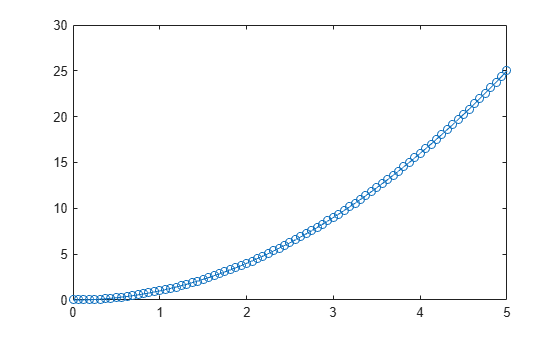
Solve the ODE

y′=2t.

Specify a time interval of [0 5] and the initial condition y0 = 0.

tspan = [0 5]; y0 = 0; [t,y] = ode78(@(t,y) 2*t, tspan, y0);

Plot the solution.

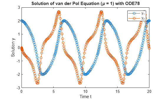
The van der Pol equation is a second-order ODE

y1′′-μ(1-y12)y1′+y1=0,

where μ>0 is a scalar parameter. Rewrite this equation as a system of first-order ODEs by making the substitution y1′=y2. The resulting system of first-order ODEs is

y1′=y2y2′=μ(1-y12)y2-y1.

The function file vdp1.m represents the van der Pol equation using μ=1. The variables y1 and y2 are the entries y(1) and y(2) of a two-element vector dydt.

function dydt = vdp1(t,y) %VDP1 Evaluate the van der Pol ODEs for mu = 1 % % See also ODE113, ODE23, ODE45.

% Jacek Kierzenka and Lawrence F. Shampine % Copyright 1984-2014 The MathWorks, Inc.

dydt = [y(2); (1-y(1)^2)*y(2)-y(1)];

Solve the ODE using the ode78 function on the time interval [0 20] with initial values [2 0]. The resulting output is a column vector of time points t and a solution array y. Each row in y corresponds to a time returned in the corresponding row of t. The first column of y corresponds to y1, and the second column corresponds to y2.

[t,y] = ode78(@vdp1,[0 20],[2; 0]);

Plot the solutions for y1 and y2 against t.

plot(t,y(:,1),'-o',t,y(:,2),'-o') title('Solution of van der Pol Equation (\mu = 1) with ODE78'); xlabel('Time t'); ylabel('Solution y'); legend('y_1','y_2')

ode78 works only with functions that use two input arguments, t and y. However, you can pass extra parameters by defining them outside the function and passing them in when you specify the function handle.

Solve the ODE

y′′=ABty.

Rewriting the equation as a first-order system yields

y1′=y2y2′=ABty1.

odefcn, a local function at the end of this example, represents this system of equations as a function that accepts four input arguments: t, y, A, and B.

function dydt = odefcn(t,y,A,B) dydt = zeros(2,1); dydt(1) = y(2); dydt(2) = (A/B)*t.*y(1); end

Solve the ODE using ode78. Specify the function handle so that it passes the predefined values for A and B to odefcn.

A = 1; B = 2; tspan = [0 5]; y0 = [0 0.01]; [t,y] = ode78(@(t,y) odefcn(t,y,A,B), tspan, y0);

Plot the results.

plot(t,y(:,1),'-o',t,y(:,2),'-.')

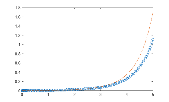
function dydt = odefcn(t,y,A,B) dydt = zeros(2,1); dydt(1) = y(2); dydt(2) = (A/B)*t.*y(1); end

Compared to ode45, the ode113, ode78, and ode89 solvers are better at solving problems with stringent error tolerances. A common situation where these solvers excel is in orbital dynamics problems, where the solution curve is smooth and requires high accuracy in each step from the solver.

The two-body problem considers two interacting masses m1 and m2 orbiting a common plane. In this example, one of the masses is significantly larger than the other. With the heavy body at the origin, the equations of motion are

x′′=-x/r3y′′=-y/r3,

where

r=x2+y2.

To solve the problem, first convert to a system of four first-order ODEs using the substitutions

y1=xy2=x′y3=yy4=y′.

The substitutions produce the first-order system

y1′=y2y2′=-y1/r3y3′=y4y4′=-y3/r3.

twobodyode, a local function included at the end of this example, codes the system of equations for the two-body problem.

function dy = twobodyode(t,y) % Two-body problem with one mass much larger than the other. r = sqrt(y(1)^2 + y(3)^2); dy = [y(2); -y(1)/r^3; y(4); -y(3)/r^3]; end

Solve the system of ODEs using ode78. Specify stringent error tolerances of 1e-13 for RelTol and 1e-14 for AbsTol.

opts = odeset('Reltol',1e-13,'AbsTol',1e-14,'Stats','on'); tspan = [0 10*pi]; y0 = [2 0 0 0.5]; [t,y] = ode78(@twobodyode, tspan, y0, opts);

341 successful steps 0 failed attempts 5797 function evaluations

plot(t,y) legend('x','x''','y','y''','Location','SouthEast') title('Position and Velocity Components')

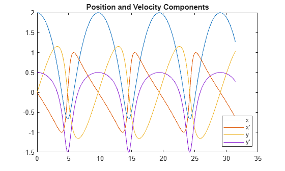
figure plot(y(:,1),y(:,3),'-o',0,0,'ro') axis equal title('Orbit of Smaller Mass')

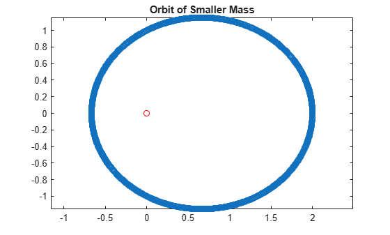
Compared to ode45, the ode78 solver is able to obtain the solution faster and with fewer steps and function evaluations.

function dy = twobodyode(t,y) % Two-body problem with one mass much larger than the other. r = sqrt(y(1)^2 + y(3)^2); dy = [y(2); -y(1)/r^3; y(4); -y(3)/r^3]; end

Input Arguments

collapse all

Data Types: function_handle

Data Types: single | double

Initial conditions, specified as a vector. y0 must be the same length as the vector output of odefun, so that y0 contains an initial condition for each equation defined in odefun.

Data Types: single | double

Output Arguments

collapse all

Solutions, returned as an array. Each row in y corresponds to the solution at the value returned in the corresponding row of t.

Time of events, returned as a column vector. The event times in te correspond to the solutions returned in ye, and ie specifies which event occurred.

Solution at time of events, returned as an array. The event times in te correspond to the solutions returned in ye, and ie specifies which event occurred.

Index of triggered event function, returned as a column vector. The event times inte correspond to the solutions returned inye, and ie specifies which event occurred.

Algorithms

ode78 is an implementation of Verner's "most efficient" Runge-Kutta 8(7) pair with a 7th-order continuous extension. The solution is advanced with the 8th-order result. The 7th-order continuous extension requires four additional evaluations ofodefun, but only on steps that require interpolation.

Extended Capabilities

expand all

Usage notes and limitations:

• All odeset option arguments must be constant.
• Code generation does not support a constant mass matrix in the options structure. Provide a mass matrix as a function.
• You must provide at least the two output arguments T andY.
• Input types must be homogeneous—all double or all single.
• Variable-sizing support must be enabled. Code generation requires dynamic memory allocation when tspan has two elements or you use event functions.

Version History

Introduced in R2021b