ss2tf - Convert state-space representation to transfer function - MATLAB (original) (raw)

Convert state-space representation to transfer function

Syntax

Description

[[b](#buh3rcg-b),[a](#buh3rcg-a)] = ss2tf([A](#buh3rcg-A),[B](#buh3rcg-B),[C](#buh3rcg-C),[D](#buh3rcg-D)) converts a state-space representation of a system into an equivalent transfer function. ss2tf returns the Laplace-transform transfer function for continuous-time systems and the Z-transform transfer function for discrete-time systems.

example

[[b](#buh3rcg-b),[a](#buh3rcg-a)] = ss2tf([A](#buh3rcg-A),[B](#buh3rcg-B),[C](#buh3rcg-C),[D](#buh3rcg-D),[ni](#buh3rcg-ni)) returns the transfer function that results when the nith input of a system with multiple inputs is excited by a unit impulse.

example

Examples

collapse all

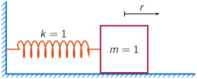
A one-dimensional discrete-time oscillating system consists of a unit mass, m, attached to a wall by a spring of unit elastic constant. A sensor samples the acceleration, a, of the mass at Fs=5 Hz.

Generate 50 time samples. Define the sampling interval Δt=1/Fs.

Fs = 5; dt = 1/Fs; N = 50; t = dt*(0:N-1);

The oscillator can be described by the state-space equations

x(k+1)=Ax(k)+Bu(k),y(k)=Cx(k)+Du(k),

where x=(rv)T is the state vector, r and v are respectively the position and velocity of the mass, and the matrices

A=(cosΔtsinΔt-sinΔtcosΔt),B=(1-cosΔtsinΔt),C=(-10),D=(1).

A = [cos(dt) sin(dt);-sin(dt) cos(dt)]; B = [1-cos(dt);sin(dt)]; C = [-1 0]; D = 1;

The system is excited with a unit impulse in the positive direction. Use the state-space model to compute the time evolution of the system starting from an all-zero initial state.

u = [1 zeros(1,N-1)];

x = [0;0]; for k = 1:N y(k) = Cx + Du(k); x = Ax + Bu(k); end

Plot the acceleration of the mass as a function of time.

stem(t,y,'filled') xlabel('t')

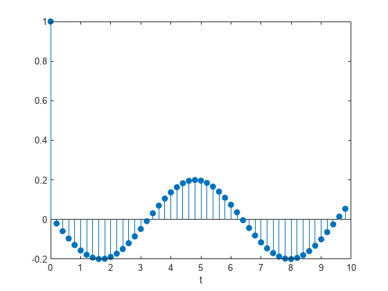
Figure contains an axes object. The axes object with xlabel t contains an object of type stem.

Compute the time-dependent acceleration using the transfer function H(z) to filter the input. Plot the result.

[b,a] = ss2tf(A,B,C,D); yt = filter(b,a,u);

stem(t,yt,'filled') xlabel('t')

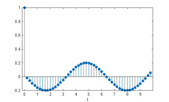
Figure contains an axes object. The axes object with xlabel t contains an object of type stem.

The transfer function of the system has an analytic expression:

H(z)=1-z-1(1+cosΔt)+z-2cosΔt1-2z-1cosΔt+z-2.

Use the expression to filter the input. Plot the response.

bf = [1 -(1+cos(dt)) cos(dt)]; af = [1 -2*cos(dt) 1]; yf = filter(bf,af,u);

stem(t,yf,'filled') xlabel('t')

Figure contains an axes object. The axes object with xlabel t contains an object of type stem.

The result is the same in all three cases.

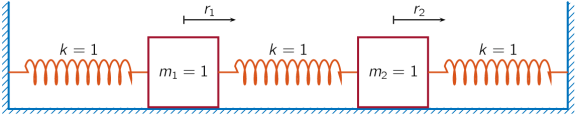
An ideal one-dimensional oscillating system consists of two unit masses, m1 and m2, confined between two walls. Each mass is attached to the nearest wall by a spring of unit elastic constant. Another such spring connects the two masses. Sensors sample a1 and a2, the accelerations of the masses, at Fs=16 Hz.

Specify a total measurement time of 16 s. Define the sampling interval Δt=1/Fs.

Fs = 16; dt = 1/Fs; N = 257; t = dt*(0:N-1);

The system can be described by the state-space model

x(n+1)=Ax(n)+Bu(n),y(n)=Cx(n)+Du(n),

where x=(r1v1r2v2)T is the state vector and ri and vi are respectively the location and the velocity of the ith mass. The input vector u=(u1u2)T and the output vector y=(a1a2)T. The state-space matrices are

A=exp(AcΔt),B=Ac-1(A-I)Bc,C=(-201010-20),D=I,

the continuous-time state-space matrices are

Ac=(0100-2010000110-20),Bc=(00100001),

and I denotes an identity matrix of the appropriate size.

Ac = [0 1 0 0; -2 0 1 0; 0 0 0 1; 1 0 -2 0]; A = expm(Ac*dt); Bc = [0 0; 1 0; 0 0; 0 1]; B = Ac(A-eye(4))*Bc; C = [-2 0 1 0; 1 0 -2 0]; D = eye(2);

The first mass, m1, receives a unit impulse in the positive direction.

ux = [1 zeros(1,N-1)]; u0 = zeros(1,N); u = [ux;u0];

Use the model to compute the time evolution of the system starting from an all-zero initial state.

x = [0 0 0 0]'; y = zeros(2,N);

for k = 1:N y(:,k) = Cx + Du(:,k); x = Ax + Bu(:,k); end

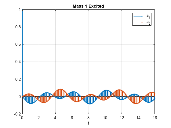
Plot the accelerations of the two masses as functions of time.

stem(t,y','.') xlabel('t') legend('a_1','a_2') title('Mass 1 Excited') grid

Figure contains an axes object. The axes object with title Mass 1 Excited, xlabel t contains 2 objects of type stem. These objects represent a_1, a_2.

Convert the system to its transfer function representation. Find the response of the system to a positive unit impulse excitation on the first mass.

[b1,a1] = ss2tf(A,B,C,D,1); y1u1 = filter(b1(1,:),a1,ux); y1u2 = filter(b1(2,:),a1,ux);

Plot the result. The transfer function gives the same response as the state-space model.

stem(t,[y1u1;y1u2]','.') xlabel('t') legend('a_1','a_2') title('Mass 1 Excited') grid

Figure contains an axes object. The axes object with title Mass 1 Excited, xlabel t contains 2 objects of type stem. These objects represent a_1, a_2.

The system is reset to its initial configuration. Now the other mass, m2, receives a unit impulse in the positive direction. Compute the time evolution of the system.

u = [u0;ux];

x = [0;0;0;0]; for k = 1:N y(:,k) = Cx + Du(:,k); x = Ax + Bu(:,k); end

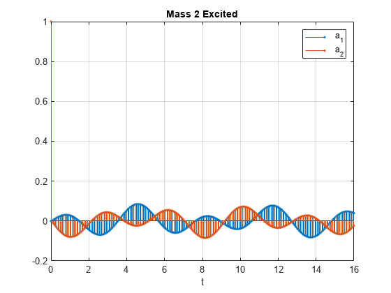
Plot the accelerations. The responses of the individual masses are switched.

stem(t,y','.') xlabel('t') legend('a_1','a_2') title('Mass 2 Excited') grid

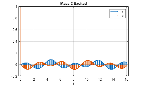
Figure contains an axes object. The axes object with title Mass 2 Excited, xlabel t contains 2 objects of type stem. These objects represent a_1, a_2.

Find the response of the system to a positive unit impulse excitation on the second mass.

[b2,a2] = ss2tf(A,B,C,D,2); y2u1 = filter(b2(1,:),a2,ux); y2u2 = filter(b2(2,:),a2,ux);

Plot the result. The transfer function gives the same response as the state-space model.

stem(t,[y2u1;y2u2]','.') xlabel('t') legend('a_1','a_2') title('Mass 2 Excited') grid

Figure contains an axes object. The axes object with title Mass 2 Excited, xlabel t contains 2 objects of type stem. These objects represent a_1, a_2.

Input Arguments

collapse all

State matrix, specified as a matrix. If the system has p inputs and q outputs and is described by n state variables, then A is _n_-by-n.