svds - Subset of singular values and vectors - MATLAB (original) (raw)

Subset of singular values and vectors

Syntax

Description

[s](#bu4i2cw-s) = svds([A](#bu4i2cw-A)) returns a vector of the six largest singular values of matrixA. This is useful when computing all of the singular values with svd is computationally expensive, such as with large sparse matrices.

example

[s](#bu4i2cw-s) = svds([A](#bu4i2cw-A),[k](#bu4i2cw-k)) returns the k largest singular values.

example

[s](#bu4i2cw-s) = svds([A](#bu4i2cw-A),[k](#bu4i2cw-k),[sigma](#bu4i2cw-sigma)) returns k singular values based on the value of sigma. For example, svds(A,k,'smallest') returns the k smallest singular values.

example

[s](#bu4i2cw-s) = svds([A](#bu4i2cw-A),[k](#bu4i2cw-k),[sigma](#bu4i2cw-sigma),[Name,Value](#namevaluepairarguments)) specifies additional options with one or more name-value pair arguments. For example, svds(A,k,sigma,'Tolerance',1e-3) adjusts the convergence tolerance for the algorithm.

[s](#bu4i2cw-s) = svds([A](#bu4i2cw-A),[k](#bu4i2cw-k),[sigma](#bu4i2cw-sigma),[opts](#bu4i2cw-opts)) specifies options using a structure.

example

[s](#bu4i2cw-s) = svds([Afun](#bu4i2cw-Afun),[n](#bu4i2cw-n),___) specifies a function handle Afun instead of a matrix. The second input n gives the size of matrix A used in Afun. You can optionally specifyk, sigma, opts, or name-value pairs as additional input arguments.

example

[[U](#bu4i2cw-U),[S](#bu4i2cw-S),[V](#bu4i2cw-V)] = svds(___) returns the left singular vectors U, diagonal matrix S of singular values, and right singular vectors V. You can use any of the input argument combinations in previous syntaxes.

example

[[U](#bu4i2cw-U),[S](#bu4i2cw-S),[V](#bu4i2cw-V),[flag](#bu4i2cw-flag)] = svds(___) also returns a convergence flag. If flag is 0, then all the singular values converged.

example

Examples

collapse all

The matrix A = delsq(numgrid('C',15)) is a symmetric positive definite matrix with singular values reasonably well-distributed in the interval (0 8). Compute the six largest singular values.

A = delsq(numgrid('C',15)); s = svds(A)

s = 6×1

Specify a second input to compute a specific number of the largest singular values.

s = 3×1

7.8666
7.7324
7.6531

The matrix A = delsq(numgrid('C',15)) is a symmetric positive definite matrix with singular values reasonably well-distributed in the interval (0 8). Compute the five smallest singular values.

A = delsq(numgrid('C',15)); s = svds(A,5,'smallest')

s = 5×1

Create a sparse 100-by-100 Neumann matrix.

C = gallery('neumann',100);

Compute the ten smallest singular values.

ss = svds(C,10,'smallest')

ss = 10×1

Compute the 10 smallest nonzero singular values. Since the matrix has a singular value that is equal to zero, the 'smallestnz' option omits it.

snz = svds(C,10,'smallestnz')

snz = 10×1

Create two matrices representing the upper-right and lower-left nonzero blocks in a sparse matrix.

n = 500; B = rand(500); C = rand(500);

Save Afun in your current directory so that it is available for use with svds.

function y = Afun(x,tflag,B,C,n) if strcmp(tflag,'notransp') y = [Bx(n+1:end); Cx(1:n)]; else y = [C'*x(n+1:end); B'*x(1:n)]; end

The function Afun uses B and C to compute either A*x or A'*x (depending on the specified flag) without actually forming the entire sparse matrix A = [zeros(n) B; C zeros(n)]. This exploits the sparsity pattern of the matrix to save memory in the computation of A*x and A'*x.

Use Afun to calculate the 10 largest singular values of A. Pass B, C, and n as additional inputs to Afun.

s = svds(@(x,tflag) Afun(x,tflag,B,C,n),[1000 1000],10)

s =

250.3248 249.9914 12.7627 12.7232 12.6988 12.6608 12.6166 12.5643 12.5419 12.4512

Directly compute the 10 largest singular values of A to compare the results.

A = [zeros(n) B; C zeros(n)]; s = svds(A,10)

s =

250.3248 249.9914 12.7627 12.7232 12.6988 12.6608 12.6166 12.5643 12.5419 12.4512

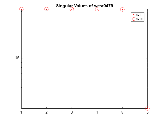
west0479 is a real-valued 479-by-479 sparse matrix. The matrix has a few large singular values, and many small singular values.

Load west0479 and store it as A.

load west0479 A = west0479;

Compute the singular value decomposition of A, returning the six largest singular values and the corresponding singular vectors. Specify a fourth output argument to check convergence of the singular values.

[U,S,V,cflag] = svds(A); cflag

cflag indicates that all of the singular values converged. The singular values are on the diagonal of the output matrix S.

s = 6×1 105 ×

Check the results by computing the full singular value decomposition of A. Convert A to a full matrix and use svd.

[U1,S1,V1] = svd(full(A));

Plot the six largest singular values of A computed by svd and svds using a logarithmic scale.

s2 = diag(S1); semilogy(s2(1:6),'r.') hold on semilogy(s,'ro','MarkerSize',10) title('Singular Values of west0479') legend('svd','svds')

Figure contains an axes object. The axes object with title Singular Values of west0479 contains 2 objects of type line. One or more of the lines displays its values using only markers These objects represent svd, svds.

Create a sparse diagonal matrix and calculate the six largest singular values.

A = diag(sparse([1e4*ones(1, 8) 1e4:-1:1])); s = svds(A)

Warning: Only 2 of the 6 requested singular values converged. Singular values that did not converge are NaN.

s = 6×1 104 ×

1.0000
0.9999
   NaN
   NaN
   NaN
   NaN

The svds algorithm produces a warning since the maximum number of iterations were performed but the tolerance could not be met.

The most effective way to address convergence problems is to increase the maximum size of the Krylov subspace used in the calculation by using a larger value for 'SubspaceDimension'. Do this by passing in the name-value pair 'SubspaceDimension' with a value of 60.

s = svds(A,6,'largest','SubspaceDimension',60)

s = 6×1 104 ×

Compute the 10 smallest singular values of a nearly singular matrix.

rng default format shortg B = spdiags([repelem([1; 1e-7], [198, 2]) ones(200, 1)], [0 1], 200, 200); s1 = svds(B,10,'smallest')

Warning: Large residual norm detected. This is likely due to bad condition of the input matrix (condition number 1.0008e+16).

s1 = 10×1

7.0888e-16

The warning indicates that svds fails to calculate the proper singular values. The failure with svds is because of the gap between the smallest and second smallest singular values. svds(...,'smallest') needs to invert B, which leads to large numerical error.

For comparison, compute the exact singular values using svd.

s = svd(full(B)); s = s(end-9:end)

s = 10×1

7.0888e-16

In order to reproduce this calculation with svds, do a QR decomposition of B. The singular values of the triangular matrix R are the same as for B.

Plot the norm of each row of R.

rownormR = sqrt(diag(R*R')); semilogy(rownormR) hold on; semilogy(size(R, 1), rownormR(end), 'ro')

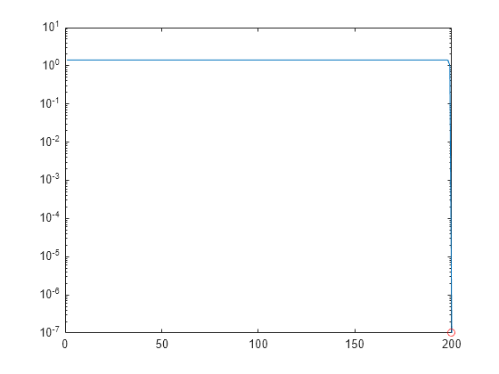
Figure contains an axes object. The axes object contains 2 objects of type line. One or more of the lines displays its values using only markers

The last entry in R is nearly zero, which causes instability in the solution.

Prevent this entry from corrupting the good parts of the solution by setting the last row of R to be exactly zero.

Use svds to find the 10 smallest singular values of R. The results are comparable to those obtained by svd.

sr = svds(R,10,'smallest')

sr = 10×1

To compute the singular vectors of B using this method, transform the left and right singular vectors using Q and the permutation vector p.

[U,S,V] = svds(R,20,'s'); U = Q*U; V(p,:) = V;

Input Arguments

collapse all

Input matrix. A is typically, but not always, a large and sparse matrix.

Data Types: single | double
Complex Number Support: Yes

Number of singular values to compute, specified as a positive scalar integer. svds returns fewer singular values than requested if either of these conditions are met:

k is larger than min(size(A))
sigma = 'smallestnz' and k is larger than the number of nonzero singular values of A

If k is too large, then svds replaces it with the maximum valid value of k.

Example: svds(A,2) returns the two largest singular values of A.

Type of singular values, specified as one of these values.

Option	Description
'largest' (default)	Largest singular values
'smallest'	Smallest singular values
'smallestnz'	Smallest nonzero singular values
scalar	Singular values closest to a scalar

Example: svds(A,k,'smallest') computes the k smallest singular values.

Example: svds(A,k,100) computes the k singular values closest to 100.

Data Types: single | double | char | string

Options structure, specified as a structure containing one or more of the fields in this table.

Note

Use of the options structure to specify options is not recommended. Use name-value pairs instead.

Option Field	Description	Name-Value Pair
tol	Convergence tolerance	'Tolerance'
maxit	Maximum number of iterations	'MaxIterations'
p	Maximum size of Krylov subspace	'SubspaceDimension'
u0	Left initial starting vector	'LeftStartVector'
v0	Right initial starting vector	'RightStartVector'
disp	Diagnostic information display level	'Display'
fail	Treatment of nonconverged singular values in the output	'FailureTreatment'

Note

svds ignores the option p when using a numeric scalar shift sigma.

Example: opts.tol = 1e-6, opts.maxit = 500 creates a structure with values set for the fields tol and maxit.

Data Types: struct

Matrix function, specified as a function handle. The function Afun must satisfy these conditions:

Afun(x,'notransp') accepts a vector x and returns the product A*x.
Afun(x,'transp') accepts a vector x and returns the product A'*x.

Note

Use function handles only in the case where sigma = 'largest' (which is the default).

Example: svds(Afun,[1000 1200])

Size of matrix A that is used by Afun, specified as a two-element size vector [m n].

Name-Value Arguments

collapse all

Specify optional pairs of arguments asName1=Value1,...,NameN=ValueN, where Name is the argument name and Value is the corresponding value. Name-value arguments must appear after other arguments, but the order of the pairs does not matter.

Before R2021a, use commas to separate each name and value, and enclose Name in quotes.

Example: s = svds(A,k,sigma,'Tolerance',1e-10,'MaxIterations',100) loosens the convergence tolerance and uses fewer iterations.

Convergence tolerance, specified as the comma-separated pair consisting of 'Tolerance' and a nonnegative real numeric scalar.

Example: s = svds(A,k,sigma,'Tolerance',1e-3)

Maximum number of algorithm iterations, specified as the comma-separated pair consisting of 'MaxIterations' and a positive integer.

Example: s = svds(A,k,sigma,'MaxIterations',350)

Maximum size of Krylov subspace, specified as the comma-separated pair consisting of 'SubspaceDimension' and a nonnegative integer. The 'SubspaceDimension' value must be greater than or equal to k + 2, wherek is the number of singular values.

For problems where svds fails to converge, increasing the value of 'SubspaceDimension' can improve the convergence behavior.

This option is ignored for numeric values ofsigma.

Example: s = svds(A,k,sigma,'SubspaceDimension',25)

Left initial starting vector, specified as the comma-separated pair consisting of 'LeftStartVector' and a numeric vector.

You can specify either'LeftStartVector' or 'RightStartVector', but not both. If neither option is specified, then for an m-by-n matrixA, the default is:

m < n — Left initial starting vector set torandn(m,1)
m >= n — Right initial starting vector set torandn(n,1)

The primary reason to specify a different random starting vector is to control the random number stream used to generate the vector.

Note

svds selects the starting vectors in a reproducible manner using a private random number stream. Changing the random number seed does_not_ affect this use of randn.

Example: s = svds(A,k,sigma,'LeftStartVector',randn(m,1)) uses a random starting vector that draws values from the global random number stream.

Data Types: single | double

Right initial starting vector, specified as the comma-separated pair consisting of 'RightStartVector' and a numeric vector.

You can specify either'LeftStartVector' or 'RightStartVector', but not both. If neither option is specified, then for an m-by-n matrixA, the default is:

m < n — Left initial starting vector set torandn(m,1)
m >= n — Right initial starting vector set torandn(n,1)

The primary reason to specify a different random starting vector is to control the random number stream used to generate the vector.

Note

svds selects the starting vectors in a reproducible manner using a private random number stream. Changing the random number seed does_not_ affect this use of randn.

Example: s = svds(A,k,sigma,'RightStartVector',randn(n,1)) uses a random starting vector that draws values from the global random number stream.

Data Types: single | double

Treatment of nonconverged singular values, specified as the comma-separated pair consisting of 'FailureTreatment' and one of the options: 'replacenan','keep', or 'drop'.

The value of 'FailureTreatment' determines how nonconverged singular values are displayed in the output.

Option	Affect on Output
'drop'	Nonconverged singular values are removed from the output, which can result insvds returning fewer singular values than requested. This value is the default for numeric values of sigma.
'replacenan'	Nonconverged singular values are replaced withNaN values. This value is the default whenever sigma is not numeric.
'keep'	Nonconverged singular values are included in the output.

Example: s = svds(A,k,sigma,'FailureTreatment','drop') removes nonconverged singular values from the output.

Data Types: char | string

Toggle for diagnostic information display, specified asfalse, true,0, or 1. Values offalse or 0 turn off the display, while values of true or 1 turn it on.

Output Arguments

collapse all

Singular values, returned as a column vector. The singular values are nonnegative real numbers listed in decreasing order.

Left singular vectors, returned as the columns of a matrix. If A is an m-by-n matrix and you request k singular values, then U is an m-by-k matrix with orthonormal columns.

Different machines, releases of MATLAB®, or parameters (such as the starting vector and subspace dimension) can produce different singular vectors that are still numerically accurate. Corresponding columns inU and V can flip their signs, since this does not affect the value of the expression A = U*S*V'.

Singular values, returned as a diagonal matrix. The diagonal elements of S are nonnegative singular values. If A is an m-by-n matrix and you request k singular values, then S is k-by-k.

Right singular vectors, returned as the columns of a matrix. IfA is an m-by-n matrix and you request k singular values, thenV is an n-by-k matrix with orthonormal columns.

Different machines, releases of MATLAB, or parameters (such as the starting vector and subspace dimension) can produce different singular vectors that are still numerically accurate. Corresponding columns inU and V can flip their signs, since this does not affect the value of the expression A = U*S*V'.

Convergence flag, returned as a scalar. A value of 0 indicates that all the singular values converged. Otherwise, not all the singular values converged.

Use of this convergence flag output suppresses warnings about failed convergence.

Tips

svdsketch is useful when you do not know ahead of time what rank to specify with svds, but you know what tolerance the approximation of the SVD should satisfy.
svds generates the default starting vectors using a private random number stream to ensure reproducibility across runs. Setting the random number generator state using rng before callingsvds does not affect the output.
Using svds is not the most efficient way to find a few singular values of small, dense matrices. For such problems, using svd(full(A)) might be quicker. For example, finding three singular values in a 500-by-500 matrix is a relatively small problem that svd can handle easily.
If svds fails to converge for a given matrix, increase the size of the Krylov subspace by increasing the value of'SubspaceDimension'. As secondary options, adjusting the maximum number of iterations ('MaxIterations') and the convergence tolerance ('Tolerance') also can help with convergence behavior.
Increasing k can sometimes improve performance, especially when the matrix has repeated singular values.

References

[1] Baglama, J. and L. Reichel, “Augmented Implicitly Restarted Lanczos Bidiagonalization Methods.” SIAM Journal on Scientific Computing. Vol. 27, 2005, pp. 19–42.

Extended Capabilities

expand all

The svds function supports GPU array input with these usage notes and limitations:

If you provide the sigma parameter, the value must be'largest'.
Input matrix A must be of typedouble.

For more information, see Run MATLAB Functions on a GPU (Parallel Computing Toolbox).

Usage notes and limitations:

If you provide the sigma parameter, the value must be'largest'.
Input matrix A must be of typedouble.

For more information, see Run MATLAB Functions with Distributed Arrays (Parallel Computing Toolbox).

Version History

Introduced before R2006a

expand all

You can specify these arguments as single precision:

A — Input matrix
sigma — Type of eigenvalues
LeftStartVector — Left initial starting vector
RightStartVector — Right initial starting vector

If you specify A, LeftStartVector, orRightStartVector as single precision, the function computes in single precision and returns outputs of type single.

If you specify only the matrix function Afun and the matrix size n as inputs, the outputs of svds are of the same precision as the output of Afun. If you also specify LeftStartVector orRightStartVector as single, then the output of Afun must also be single.

Reproducibility
Calling svds multiple times in succession now produces the same result. To change this behavior:
- In R2017a or earlier, set the u0 orv0 field of the options structure to a random vector.
- In R2017b or later, prefer setting'LeftStartVector' or'RightStartVector' to a random vector.