fsolve - Solve system of nonlinear equations - MATLAB (original) (raw)
Solve system of nonlinear equations
Syntax
Description
Nonlinear system solver
Solves a problem specified by
F(x) = 0
for x, where F(x) is a function that returns a vector value.
x is a vector or a matrix; see Matrix Arguments.
[x](#buta%5F%5Fs%5Fsep%5Fshared-x) = fsolve([fun](#buta%5F%5Fs-fun),[x0](#buta%5F%5Fs-x0)) starts at x0 and tries to solve the equations fun(x) = 0, an array of zeros.
[x](#buta%5F%5Fs%5Fsep%5Fshared-x) = fsolve([fun](#buta%5F%5Fs-fun),[x0](#buta%5F%5Fs-x0),[options](#buta%5F%5Fs-options)) solves the equations with the optimization options specified in options. Use optimoptions to set these options.
[[x](#buta%5F%5Fs%5Fsep%5Fshared-x),[fval](#buta%5F%5Fs-fval)] = fsolve(___), for any syntax, returns the value of the objective function fun at the solution x.
[[x](#buta%5F%5Fs%5Fsep%5Fshared-x),[fval](#buta%5F%5Fs-fval),[exitflag](#buta%5F%5Fs-exitflag),[output](#buta%5F%5Fs-output)] = fsolve(___) additionally returns a value exitflag that describes the exit condition of fsolve, and a structure output with information about the optimization process.
[[x](#buta%5F%5Fs%5Fsep%5Fshared-x),[fval](#buta%5F%5Fs-fval),[exitflag](#buta%5F%5Fs-exitflag),[output](#buta%5F%5Fs-output),[jacobian](#buta%5F%5Fs%5Fsep%5Fshared-jacobian)] = fsolve(___) returns the Jacobian of fun at the solution x.
Examples
This example shows how to solve two nonlinear equations in two variables. The equations are
e-e-(x1+x2)=x2(1+x12)x1cos(x2)+x2sin(x1)=12.
Convert the equations to the form F(x)=0.
e-e-(x1+x2)-x2(1+x12)=0x1cos(x2)+x2sin(x1)-12=0.
The root2d.m function, which is available when you run this example, computes the values.
function F = root2d(x)
F(1) = exp(-exp(-(x(1)+x(2)))) - x(2)*(1+x(1)^2); F(2) = x(1)*cos(x(2)) + x(2)*sin(x(1)) - 0.5;
Solve the system of equations starting at the point [0,0].
fun = @root2d; x0 = [0,0]; x = fsolve(fun,x0)
Equation solved.
fsolve completed because the vector of function values is near zero as measured by the value of the function tolerance, and the problem appears regular as measured by the gradient.
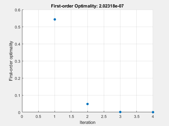
Examine the solution process for a nonlinear system.
Set options to have no display and a plot function that displays the first-order optimality, which should converge to 0 as the algorithm iterates.
options = optimoptions('fsolve','Display','none','PlotFcn',@optimplotfirstorderopt);
The equations in the nonlinear system are
e-e-(x1+x2)=x2(1+x12)x1cos(x2)+x2sin(x1)=12.
Convert the equations to the form F(x)=0.
e-e-(x1+x2)-x2(1+x12)=0x1cos(x2)+x2sin(x1)-12=0.
The root2d function computes the left-hand side of these two equations.
function F = root2d(x)
F(1) = exp(-exp(-(x(1)+x(2)))) - x(2)*(1+x(1)^2); F(2) = x(1)*cos(x(2)) + x(2)*sin(x(1)) - 0.5;
Solve the nonlinear system starting from the point [0,0] and observe the solution process.
fun = @root2d; x0 = [0,0]; x = fsolve(fun,x0,options)

You can parameterize equations as described in the topic Passing Extra Parameters. For example, the paramfun helper function at the end of this example creates the following equation system parameterized by c:
2x1+x2=exp(cx1)-x1+2x2=exp(cx2).
To solve the system for a particular value, in this case c=-1, set c in the workspace and create an anonymous function in x from paramfun.
c = -1; fun = @(x)paramfun(x,c);
Solve the system starting from the point x0 = [0 1].
x0 = [0 1]; x = fsolve(fun,x0)
Equation solved.
fsolve completed because the vector of function values is near zero as measured by the value of the function tolerance, and the problem appears regular as measured by the gradient.
To solve for a different value of c, enter c in the workspace and create the fun function again, so it has the new c value.
c = -2; fun = @(x)paramfun(x,c); % fun now has the new c value x = fsolve(fun,x0)
Equation solved.
fsolve completed because the vector of function values is near zero as measured by the value of the function tolerance, and the problem appears regular as measured by the gradient.
Helper Function
This code creates the paramfun helper function.
function F = paramfun(x,c) F = [ 2x(1) + x(2) - exp(cx(1)) -x(1) + 2x(2) - exp(cx(2))]; end
Create a problem structure for fsolve and solve the problem.
Solve the same problem as in Solution with Nondefault Options, but formulate the problem using a problem structure.
Set options for the problem to have no display and a plot function that displays the first-order optimality, which should converge to 0 as the algorithm iterates.
problem.options = optimoptions('fsolve','Display','none','PlotFcn',@optimplotfirstorderopt);
The equations in the nonlinear system are
e-e-(x1+x2)=x2(1+x12)x1cos(x2)+x2sin(x1)=12.
Convert the equations to the form F(x)=0.
e-e-(x1+x2)-x2(1+x12)=0x1cos(x2)+x2sin(x1)-12=0.
The root2d function computes the left-hand side of these two equations.
function F = root2d(x)
F(1) = exp(-exp(-(x(1)+x(2)))) - x(2)*(1+x(1)^2); F(2) = x(1)*cos(x(2)) + x(2)*sin(x(1)) - 0.5;
Create the remaining fields in the problem structure.
problem.objective = @root2d; problem.x0 = [0,0]; problem.solver = 'fsolve';
Solve the problem.
This example returns the iterative display showing the solution process for the system of two equations and two unknowns
2x1-x2=e-x1-x1+2x2=e-x2.
Rewrite the equations in the form F(x) = 0:
2x1-x2-e-x1=0-x1+2x2-e-x2=0.
Start your search for a solution at x0 = [-5 -5].
First, write a function that computes F, the values of the equations at x.
F = @(x) [2x(1) - x(2) - exp(-x(1)); -x(1) + 2x(2) - exp(-x(2))];
Create the initial point x0.
Set options to return iterative display.
options = optimoptions('fsolve','Display','iter');
Solve the equations.
[x,fval] = fsolve(F,x0,options)
Norm of First-order Trust-regionIteration Func-count ||f(x)||^2 step optimality radius 0 3 47071.2 2.29e+04 1 1 6 12003.4 1 5.75e+03 1 2 9 3147.02 1 1.47e+03 1 3 12 854.452 1 388 1 4 15 239.527 1 107 1 5 18 67.0412 1 30.8 1 6 21 16.7042 1 9.05 1 7 24 2.42788 1 2.26 1 8 27 0.032658 0.759511 0.206 2.5 9 30 7.03149e-06 0.111927 0.00294 2.5 10 33 3.29525e-13 0.00169132 6.36e-07 2.5
Equation solved.
fsolve completed because the vector of function values is near zero as measured by the value of the function tolerance, and the problem appears regular as measured by the gradient.
fval = 2×1 10-6 ×
-0.4059 -0.4059
The iterative display shows f(x), which is the square of the norm of the function F(x). This value decreases to near zero as the iterations proceed. The first-order optimality measure likewise decreases to near zero as the iterations proceed. These entries show the convergence of the iterations to a solution. For the meanings of the other entries, see Iterative Display.
The fval output gives the function value F(x), which should be zero at a solution (to within the FunctionTolerance tolerance).
Find a matrix X that satisfies
X*X*X=[1234],
starting at the point x0 = [1,1;1,1]. Create an anonymous function that calculates the matrix equation and create the point x0.
fun = @(x)xxx - [1,2;3,4]; x0 = ones(2);
Set options to have no display.
options = optimoptions('fsolve','Display','off');
Examine the fsolve outputs to see the solution quality and process.
[x,fval,exitflag,output] = fsolve(fun,x0,options)
x = 2×2
-0.1291 0.8602 1.2903 1.1612
fval = 2×2 10-9 ×
-0.2742 0.1258 0.1876 -0.0864
output = struct with fields: iterations: 11 funcCount: 52 algorithm: 'trust-region-dogleg' firstorderopt: 4.0197e-10 message: 'Equation solved.↵↵fsolve completed because the vector of function values is near zero↵as measured by the value of the function tolerance, and↵the problem appears regular as measured by the gradient.↵↵↵↵Equation solved. The sum of squared function values, r = 1.336702e-19, is less than↵sqrt(options.FunctionTolerance) = 1.000000e-03. The relative norm of the gradient of r,↵4.019681e-10, is less than options.OptimalityTolerance = 1.000000e-06.'
The exit flag value 1 indicates that the solution is reliable. To verify this manually, calculate the residual (sum of squares of fval) to see how close it is to zero.
This small residual confirms that x is a solution.
You can see in the output structure how many iterations and function evaluations fsolve performed to find the solution.
Input Arguments
Nonlinear equations to solve, specified as a function handle or function name. fun is a function that accepts a vector x and returns a vector F, the nonlinear equations evaluated at x. The equations to solve are F = 0 for all components of F. The function fun can be specified as a function handle for a file
where myfun is a MATLAB® function such as
function F = myfun(x) F = ... % Compute function values at x
fun can also be a function handle for an anonymous function.
x = fsolve(@(x)sin(x.*x),x0);
fsolve passes x to your objective function in the shape of the x0 argument. For example, if x0 is a 5-by-3 array, then fsolve passes x to fun as a 5-by-3 array.
If the Jacobian can also be computed and the'SpecifyObjectiveGradient' option istrue, set by
options = optimoptions('fsolve','SpecifyObjectiveGradient',true)
the function fun must return, in a second output argument, the Jacobian value J, a matrix, at x.
If fun returns a vector (matrix) of m components and x has length n, where n is the length of x0, the Jacobian J is an m-by-n matrix where J(i,j) is the partial derivative of F(i) with respect to x(j). (The Jacobian J is the transpose of the gradient of F.)
Example: fun = @(x)x*x*x-[1,2;3,4]
Data Types: char | function_handle | string
Initial point, specified as a real vector or real array. fsolve uses the number of elements in and size of x0 to determine the number and size of variables that fun accepts.
Example: x0 = [1,2,3,4]
Data Types: double
Optimization options, specified as the output of optimoptions or a structure such as optimset returns.
Some options apply to all algorithms, and others are relevant for particular algorithms. See Optimization Options Reference for detailed information.
Some options are absent from theoptimoptions display. These options appear in italics in the following table. For details, see View Optimization Options.
| All Algorithms | |
|---|---|
| Algorithm | Choose between 'trust-region-dogleg' (default), 'trust-region', and 'levenberg-marquardt'.The Algorithm option specifies a preference for which algorithm to use. It is only a preference because for the trust-region algorithm, the nonlinear system of equations cannot be underdetermined; that is, the number of equations (the number of elements of F returned by fun) must be at least as many as the length of x. Similarly, for the trust-region-dogleg algorithm, the number of equations must be the same as the length of x. fsolve uses the Levenberg-Marquardt algorithm when the selected algorithm is unavailable. For more information on choosing the algorithm, see Choosing the Algorithm.To set some algorithm options using optimset instead of optimoptions:Algorithm — Set the algorithm to 'trust-region-reflective' instead of 'trust-region'.InitDamping — Set the initial Levenberg-Marquardt parameter λ by setting Algorithm to a cell array such as {'levenberg-marquardt',.005}. |
| CheckGradients | Compare user-supplied derivatives (gradients of objective or constraints) to finite-differencing derivatives. The choices are true or the defaultfalse.Foroptimset, the name isDerivativeCheck and the values are 'on' or 'off'. See Current and Legacy Option Names.The CheckGradients option will be removed in a future release. To check derivatives, use the checkGradients function. |
| Diagnostics | Display diagnostic information about the function to be minimized or solved. The choices are 'on' or the default 'off'. |
| DiffMaxChange | Maximum change in variables for finite-difference gradients (a positive scalar). The default is Inf. |
| DiffMinChange | Minimum change in variables for finite-difference gradients (a positive scalar). The default is 0. |
| Display | Level of display (see Iterative Display): 'off' or 'none' displays no output.'iter' displays output at each iteration, and gives the default exit message.'iter-detailed' displays output at each iteration, and gives the technical exit message.'final' (default) displays just the final output, and gives the default exit message.'final-detailed' displays just the final output, and gives the technical exit message. |
| FiniteDifferenceStepSize | Scalar or vector step size factor for finite differences. When you set FiniteDifferenceStepSize to a vector v, the forward finite differences delta aredelta = v.*sign′(x).*max(abs(x),TypicalX);where sign′(x) = sign(x) except sign′(0) = 1. Central finite differences aredelta = v.*max(abs(x),TypicalX);A scalar FiniteDifferenceStepSize expands to a vector. The default is sqrt(eps) for forward finite differences, and eps^(1/3) for central finite differences.For optimset, the name isFinDiffRelStep. See Current and Legacy Option Names. |
| FiniteDifferenceType | Finite differences, used to estimate gradients, are either 'forward' (default), or 'central' (centered). 'central' takes twice as many function evaluations, but should be more accurate.The algorithm is careful to obey bounds when estimating both types of finite differences. So, for example, it could take a backward, rather than a forward, difference to avoid evaluating at a point outside bounds. For optimset, the name isFinDiffType. See Current and Legacy Option Names. |
| FunctionTolerance | Termination tolerance on the function value, a nonnegative scalar. The default is 1e-6. SeeTolerances and Stopping Criteria.For optimset, the name is TolFun. See Current and Legacy Option Names. |
| FunValCheck | Check whether objective function values are valid. 'on' displays an error when the objective function returns a value that is complex, Inf, or NaN. The default, 'off', displays no error. |
| MaxFunctionEvaluations | Maximum number of function evaluations allowed, a nonnegative integer. The default is100*numberOfVariables for the'trust-region-dogleg' and'trust-region' algorithms, and200*numberOfVariables for the'levenberg-marquardt' algorithm. See Tolerances and Stopping Criteria and Iterations and Function Counts.For optimset, the name is MaxFunEvals. See Current and Legacy Option Names. |
| MaxIterations | Maximum number of iterations allowed, a nonnegative integer. The default is 400. See Tolerances and Stopping Criteria and Iterations and Function Counts.For optimset, the name is MaxIter. See Current and Legacy Option Names. |
| OptimalityTolerance | Termination tolerance on the first-order optimality (a nonnegative scalar). The default is 1e-6. See First-Order Optimality Measure.Internally, the 'levenberg-marquardt' algorithm uses an optimality tolerance (stopping criterion) of 1e-4 times FunctionTolerance and does not use OptimalityTolerance. |
| OutputFcn | Specify one or more user-defined functions that an optimization function calls at each iteration. Pass a function handle or a cell array of function handles. The default is none ([]). See Output Function and Plot Function Syntax. |
| PlotFcn | Plots various measures of progress while the algorithm executes; select from predefined plots or write your own. Pass a built-in plot function name, a function handle, or a cell array of built-in plot function names or function handles. For custom plot functions, pass function handles. The default is none ([]): 'optimplotx' plots the current point.'optimplotfunccount' plots the function count.'optimplotfval' plots the function value.'optimplotstepsize' plots the step size.'optimplotfirstorderopt' plots the first-order optimality measure.Custom plot functions use the same syntax as output functions. See Output Functions for Optimization Toolbox and Output Function and Plot Function Syntax.Foroptimset, the name isPlotFcns. See Current and Legacy Option Names. |
| SpecifyObjectiveGradient | If true, fsolve uses a user-defined Jacobian (defined in fun), or Jacobian information (when using JacobianMultiplyFcn), for the objective function. If false (default), fsolve approximates the Jacobian using finite differences. For optimset, the name isJacobian and the values are'on' or 'off'. See Current and Legacy Option Names. |
| StepTolerance | Termination tolerance on x, a nonnegative scalar. The default is 1e-6. SeeTolerances and Stopping Criteria.For optimset, the name is TolX. See Current and Legacy Option Names. |
| TypicalX | Typical x values. The number of elements in TypicalX is equal to the number of elements in x0, the starting point. The default value is ones(numberofvariables,1). fsolve uses TypicalX for scaling finite differences for gradient estimation. The trust-region-dogleg algorithm uses TypicalX as the diagonal terms of a scaling matrix. |
| UseParallel | When true, fsolve estimates gradients in parallel. Disable by setting to the default, false. See Parallel Computing. |
| trust-region Algorithm | |
| JacobianMultiplyFcn | Jacobian multiply function, specified as a function handle. For large-scale structured problems, this function computes the Jacobian matrix product J*Y,J'*Y, orJ'*(J*Y) without actually formingJ. The function is of the formW = jmfun(Jinfo,Y,flag)whereJinfo contains data used to compute J*Y (orJ'*Y, orJ'*(J*Y)). The first argumentJinfo is the second argument returned by the objective functionfun, for example, in[F,Jinfo] = fun(x)Y is a matrix that has the same number of rows as there are dimensions in the problem. flag determines which product to compute:If flag == 0,W = J'*(J*Y). If flag > 0, W = J*Y.If flag < 0, W = J'*Y. In each case, J is not formed explicitly. fsolve usesJinfo to compute the preconditioner. See Passing Extra Parameters for information on how to supply values for any additional parametersjmfun needs.Note'SpecifyObjectiveGradient' must be set to true forfsolve to passJinfo fromfun tojmfun.See Minimization with Dense Structured Hessian, Linear Equalities for a similar example.Foroptimset, the name isJacobMult. See Current and Legacy Option Names. |
| JacobPattern | Sparsity pattern of the Jacobian for finite differencing. Set JacobPattern(i,j) = 1 when fun(i) depends on x(j). Otherwise, set JacobPattern(i,j) = 0. In other words, JacobPattern(i,j) = 1 when you can have ∂fun(i)/∂x(j) ≠ 0.Use JacobPattern when it is inconvenient to compute the Jacobian matrix J in fun, though you can determine (say, by inspection) when fun(i) depends on x(j). fsolve can approximate J via sparse finite differences when you give JacobPattern.In the worst case, if the structure is unknown, do not set JacobPattern. The default behavior is as if JacobPattern is a dense matrix of ones. Then fsolve computes a full finite-difference approximation in each iteration. This can be very expensive for large problems, so it is usually better to determine the sparsity structure. |
| MaxPCGIter | Maximum number of PCG (preconditioned conjugate gradient) iterations, a positive scalar. The default is max(1,floor(numberOfVariables/2)). For more information, see Equation Solving Algorithms. |
| PrecondBandWidth | Upper bandwidth of preconditioner for PCG, a nonnegative integer. The default PrecondBandWidth is Inf, which means a direct factorization (Cholesky) is used rather than the conjugate gradients (CG). The direct factorization is computationally more expensive than CG, but produces a better quality step towards the solution. Set PrecondBandWidth to 0 for diagonal preconditioning (upper bandwidth of 0). For some problems, an intermediate bandwidth reduces the number of PCG iterations. |
| SubproblemAlgorithm | Determines how the iteration step is calculated. The default, 'factorization', takes a slower but more accurate step than 'cg'. See Trust-Region Algorithm. |
| TolPCG | Termination tolerance on the PCG iteration, a positive scalar. The default is 0.1. |
| Levenberg-Marquardt Algorithm | |
| InitDamping | Initial value of the Levenberg-Marquardt parameter, a positive scalar. Default is 1e-2. For details, see Levenberg-Marquardt Method. |
| ScaleProblem | 'jacobian' can sometimes improve the convergence of a poorly scaled problem. The default is 'none'. |
Example: options = optimoptions('fsolve','FiniteDifferenceType','central')
Problem structure, specified as a structure with the following fields:
| Field Name | Entry |
|---|---|
| objective | Objective function |
| x0 | Initial point for x |
| solver | 'fsolve' |
| options | Options created with optimoptions |
Data Types: struct
Output Arguments
Solution, returned as a real vector or real array. The size of x is the same as the size of x0. Typically, x is a local solution to the problem when exitflag is positive. For information on the quality of the solution, see When the Solver Succeeds.
Objective function value at the solution, returned as a real vector. Generally,fval = fun(x).
Reason fsolve stopped, returned as an integer.
| 1 | Equation solved. First-order optimality is small. |
|---|---|
| 2 | Equation solved. Change in x smaller than the specified tolerance, or Jacobian at x is undefined. |
| 3 | Equation solved. Change in residual smaller than the specified tolerance. |
| 4 | Equation solved. Magnitude of search direction smaller than specified tolerance. |
| 0 | Number of iterations exceeded options.MaxIterations or number of function evaluations exceeded options.MaxFunctionEvaluations. |
| -1 | Output function or plot function stopped the algorithm. |
| -2 | Equation not solved. The exit message can have more information. |
| -3 | Equation not solved. Trust region radius became too small (trust-region-dogleg algorithm). |
Information about the optimization process, returned as a structure with fields:
| iterations | Number of iterations taken |
|---|---|
| funcCount | Number of function evaluations |
| algorithm | Optimization algorithm used |
| cgiterations | Total number of PCG iterations ('trust-region' algorithm only) |
| stepsize | Final displacement in x (not in 'trust-region-dogleg') |
| firstorderopt | Measure of first-order optimality |
| message | Exit message |
Limitations
- The function to be solved must be continuous.
- When successful,
fsolveonly gives one root. - The default trust-region dogleg method can only be used when the system of equations is square, i.e., the number of equations equals the number of unknowns. For the Levenberg-Marquardt method, the system of equations need not be square.
More About
The next few items list the possible enhanced exit messages fromfsolve. Enhanced exit messages give a link for more information as the first sentence of the message.
The initial point seems to be a solution of the equation, because the sum of squares of function values is less than the square root of the FunctionTolerance tolerance. The size of the gradient of the sum of squares is also less than OptimalityTolerance (1e-4*OptimalityTolerance for the Levenberg-Marquardt algorithm).
For suggestions on how to proceed, see Final Point Equals Initial Point.
The solver found a point where the sum of squares of function values is less than the square root of the FunctionTolerance tolerance. However, the last step was less than the StepTolerance tolerance, indicating the function may be changing rapidly, or that the function is not smooth near the final point. This is the meaning of stalled.
For suggestions on how to proceed, see Local Minimum Possible.
The solver found a point where the sum of squares of function values is less than the square root of the FunctionTolerance tolerance. However, the sum of squares changed very little in the last step, even though the gradient of the sum was larger than OptimalityTolerance (1e-4*OptimalityTolerance for the Levenberg-Marquardt algorithm). This can indicate that the reported point is not near a solution.
For suggestions on how to proceed, see Local Minimum Possible.
The next few items contain definitions for terms in the fsolve exit messages.
To solve a system of equations F(x) = 0, the solver generally attempts to minimize the sum of squared function values r = Σ(Fi(x))2. Both r and ∇r should be zero at a solution.
Generally, a tolerance is a threshold which, if crossed, stops the iterations of a solver. For more information on tolerances, see Tolerances and Stopping Criteria.
The tolerance called OptimalityTolerance relates to the first-order optimality measure. Iterations end when the first-order optimality measure is less than OptimalityTolerance.
The first-order optimality measure is the size of the gradient of the sum of squares of function values. This should be zero at the root of a smooth function.
The function tolerance calledFunctionTolerance relates to the size of the latest change in sum of squares of function values.

StepTolerance is a tolerance for the size of the last step, meaning the size of the change in location wherefsolve was evaluated.
The problem appears to be regular means the size of the gradient of the sum of squares of function values is less than the OptimalityTolerance tolerance (1e-4*OptimalityTolerance for the Levenberg-Marquardt algorithm).
The solver was unable to reduce the sum of squares of function values to below the square root of the FunctionTolerance tolerance. Its last iteration did not reduce the sum of squares enough to warrant further attempts.
For suggestions on how to proceed, see fsolve Could Not Solve Equation.
The trust region is too small to continue. This could be because the sum of squares of function values is not close to a quadratic model. For more information, see Trust-Region-Dogleg Algorithm.
The trust region is too small to continue. This could be because the sum of squares of function values is not close to a quadratic model. For more information, see Trust-Region-Dogleg Algorithm.
The Levenberg-Marquardt regularization parameter is related to the inverse of a trust-region radius. It becomes large when the sum of squares of function values is not close to a quadratic model. For more information, see Levenberg-Marquardt Method.
Tips
- For large problems, meaning those with thousands of variables or more, save memory (and possibly save time) by setting the
Algorithmoption to'trust-region'and theSubproblemAlgorithmoption to'cg'.
Algorithms
The Levenberg-Marquardt and trust-region methods are based on the nonlinear least-squares algorithms also used in lsqnonlin. Use one of these methods if the system may not have a zero. The algorithm still returns a point where the residual is small. However, if the Jacobian of the system is singular, the algorithm might converge to a point that is not a solution of the system of equations (see Limitations).
- By default
fsolvechooses the trust-region dogleg algorithm. The algorithm is a variant of the Powell dogleg method described in [8]. It is similar in nature to the algorithm implemented in [7]. See Trust-Region-Dogleg Algorithm. - The trust-region algorithm is a subspace trust-region method and is based on the interior-reflective Newton method described in [1] and [2]. Each iteration involves the approximate solution of a large linear system using the method of preconditioned conjugate gradients (PCG). See Trust-Region Algorithm.
- The Levenberg-Marquardt method is described in references [4], [5], and [6]. See Levenberg-Marquardt Method.
Alternative Functionality
App
The Optimize Live Editor task provides a visual interface for fsolve.
References
[1] Coleman, T.F. and Y. Li, “An Interior, Trust Region Approach for Nonlinear Minimization Subject to Bounds,” SIAM Journal on Optimization, Vol. 6, pp. 418-445, 1996.
[2] Coleman, T.F. and Y. Li, “On the Convergence of Reflective Newton Methods for Large-Scale Nonlinear Minimization Subject to Bounds,” Mathematical Programming, Vol. 67, Number 2, pp. 189-224, 1994.
[3] Dennis, J. E. Jr., “Nonlinear Least-Squares,” State of the Art in Numerical Analysis, ed. D. Jacobs, Academic Press, pp. 269-312.
[4] Levenberg, K., “A Method for the Solution of Certain Problems in Least-Squares,” Quarterly Applied Mathematics 2, pp. 164-168, 1944.
[5] Marquardt, D., “An Algorithm for Least-squares Estimation of Nonlinear Parameters,” SIAM Journal Applied Mathematics, Vol. 11, pp. 431-441, 1963.
[6] Moré, J. J., “The Levenberg-Marquardt Algorithm: Implementation and Theory,” Numerical Analysis, ed. G. A. Watson, Lecture Notes in Mathematics 630, Springer Verlag, pp. 105-116, 1977.
[7] Moré, J. J., B. S. Garbow, and K. E. Hillstrom, User Guide for MINPACK 1, Argonne National Laboratory, Rept. ANL-80-74, 1980.
[8] Powell, M. J. D., “A Fortran Subroutine for Solving Systems of Nonlinear Algebraic Equations,” Numerical Methods for Nonlinear Algebraic Equations, P. Rabinowitz, ed., Ch.7, 1970.
Extended Capabilities
fsolvesupports code generation using either the codegen (MATLAB Coder) function or the MATLAB Coder™ app. You must have a MATLAB Coder license to generate code.- The target hardware must support standard double-precision floating-point computations. You cannot generate code for single-precision or fixed-point computations.
- Code generation targets do not use the same math kernel libraries as MATLAB solvers. Therefore, code generation solutions can vary from solver solutions, especially for poorly conditioned problems.
- All code for generation must be MATLAB code. In particular, you cannot use a custom black-box function as an objective function for
fsolve. You can usecoder.cevalto evaluate a custom function coded in C or C++. However, the custom function must be called in a MATLAB function. fsolvedoes not support the problem argument for code generation.
[x,fval] = fsolve(problem) % Not supported- You must specify the objective function by using function handles, not strings or character names.
x = fsolve(@fun,x0,options) % Supported
% Not supported: fsolve('fun',...) or fsolve("fun",...) - For advanced code optimization involving embedded processors, you also need an Embedded Coder® license.
- You must include options for
fsolveand specify them using optimoptions. The options must include theAlgorithmoption, set to'levenberg-marquardt'.
options = optimoptions('fsolve','Algorithm','levenberg-marquardt');
[x,fval,exitflag] = fsolve(fun,x0,options); - Code generation supports these options:
Algorithm— Must be'levenberg-marquardt'FiniteDifferenceStepSizeFiniteDifferenceTypeFunctionToleranceMaxFunctionEvaluationsMaxIterationsSpecifyObjectiveGradientStepToleranceTypicalX
- Generated code has limited error checking for options. The recommended way to update an option is to use
optimoptions, not dot notation.
opts = optimoptions('fsolve','Algorithm','levenberg-marquardt');
opts = optimoptions(opts,'MaxIterations',1e4); % Recommended
opts.MaxIterations = 1e4; % Not recommended - Do not load options from a file. Doing so can cause code generation to fail. Instead, create options in your code.
- Usually, if you specify an option that is not supported, the option is silently ignored during code generation. However, if you specify a plot function or output function by using dot notation, code generation can issue an error. For reliability, specify only supported options.
- Because output functions and plot functions are not supported, solvers do not return the exit flag –1.
For an example, see Generate Code for fsolve.
Version History
Introduced before R2006a
The syntax for the JacobianMultiplyFcn option is
W = jmfun(Jinfo, Y, flag)
The Jinfo data, which MATLAB passes to your function jmfun, can now be of any data type. For example, you can now have Jinfo be a structure. In previous releases, Jinfo had to be a standard double array.
The Jinfo data is the second output of your objective function:
The CheckGradients option will be removed in a future release. To check the first derivatives of objective functions or nonlinear constraint functions, use the checkGradients function.