evaluate - Evaluate optimization expression or objectives and constraints in

        problem - MATLAB ([original](https://in.mathworks.com/help/optim/ug/optim.problemdef.optimizationexpression.evaluate.html)) ([raw](?raw))

Evaluate optimization expression or objectives and constraints in problem

Syntax

Description

Use evaluate to find the numeric value of an optimization expression at a point, or to find the values of objective and constraint expressions in an optimization problem, equation problem, or optimization constraint at a set of points.

[val](#d126e95773) = evaluate([expr](#d126e95560),[pt](#mw%5F044b9d71-d216-40f2-a717-b86a7536fabd%5Fsep%5Fmw%5Ff2b0ef39-0511-44a6-943d-b8df4c6a1a7e)) returns the value of the optimization expression expr at the value pt.

example

[val](#d126e95773) = evaluate([cons](#mw%5F044b9d71-d216-40f2-a717-b86a7536fabd%5Fsep%5Fmw%5Fa3dcab01-b74a-493e-8e2d-b960cc26dc1b),[pt](#mw%5F044b9d71-d216-40f2-a717-b86a7536fabd%5Fsep%5Fmw%5Ff2b0ef39-0511-44a6-943d-b8df4c6a1a7e)) returns the value of the constraint expression cons at the valuept.

example

[val](#d126e95773) = evaluate([prob](#mw%5F044b9d71-d216-40f2-a717-b86a7536fabd%5Fsep%5Fmw%5F97ec1311-13a3-4b88-889c-fa9152597c41),[pts](#mw%5F044b9d71-d216-40f2-a717-b86a7536fabd%5Fsep%5Fmw%5Ff575f25a-47c3-4b9a-9ff6-935fc356cf2b)) returns the values of the objective and constraint functions inprob at the points in pts.

example

Examples

collapse all

Create an optimization expression of two variables.

x = optimvar("x",3,2); y = optimvar("y",1,2); expr = sum(x,1) - 2*y;

Evaluate the expression at a point.

xmat = [3,-1; 0,1; 2,6]; sol.x = xmat; sol.y = [4,-3]; val = evaluate(expr,sol)

Create two optimization variables x and y and a 3-by-2 constraint expression in those variables.

x = optimvar("x"); y = optimvar("y"); cons = optimconstr(3,2); cons(1,1) = x^2 + y^2/4 <= 2; cons(1,2) = x^4 - y^4 <= -x^2 - y^2; cons(2,1) = x^23 + y^2 <= 2; cons(2,2) = x + y <= 3; cons(3,1) = xy + x^2 + y^2 <= 5; cons(3,2) = x^3 + y^3 <= 8;

Evaluate the constraint expressions at the point x=1, y=-1. The value of an expression L <= R is L - R.

x0.x = 1; x0.y = -1; val = evaluate(cons,x0)

val = 3×2

-0.7500 2.0000 2.0000 -3.0000 -4.0000 -8.0000

Solve a linear programming problem.

x = optimvar('x'); y = optimvar('y'); prob = optimproblem; prob.Objective = -x -y/3; prob.Constraints.cons1 = x + y <= 2; prob.Constraints.cons2 = x + y/4 <= 1; prob.Constraints.cons3 = x - y <= 2; prob.Constraints.cons4 = x/4 + y >= -1; prob.Constraints.cons5 = x + y >= 1; prob.Constraints.cons6 = -x + y <= 2;

sol = solve(prob)

Solving problem using linprog.

Optimal solution found.

sol = struct with fields: x: 0.6667 y: 1.3333

Find the value of the objective function at the solution.

val = evaluate(prob.Objective,sol)

Create an optimization problem with several linear and nonlinear constraints.

x = optimvar("x"); y = optimvar("y"); obj = (10*(y - x^2))^2 + (1 - x)^2; cons1 = x^2 + y^2 <= 1; cons2 = x + y >= 0; cons3 = y <= sin(x); cons4 = 2x + 3y <= 2.5; prob = optimproblem(Objective=obj); prob.Constraints.cons1 = cons1; prob.Constraints.cons2 = cons2; prob.Constraints.cons3 = cons3; prob.Constraints.cons4 = cons4;

Create 100 test points randomly.

rng default % For reproducibility xvals = randn(1,100); yvals = randn(1,100);

Convert the points to an OptimizationValues object for the problem.

pts = optimvalues(prob,x=xvals,y=yvals);

Evaluate the objective and constraint functions at the points pts.

val = evaluate(prob,pts);

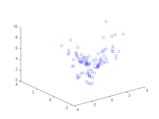
The objective function values are stored in val.Objective, and the constraint function values are stored in val.cons1 through val.cons4. Plot the log of 1 plus the objective function values.

figure plot3(xvals,yvals,log(1 + val.Objective),"bo")

Figure contains an axes object. The axes contains a line object which displays its values using only markers.

Plot the values of the constraints cons1 and cons4. Recall that constraints are satisfied when they evaluate to a nonpositive number. Plot the nonpositive values with circles and the positive values with x marks.

neg1 = val.cons1 <= 0; pos1 = val.cons1 > 0; neg4 = val.cons4 <= 0; pos4 = val.cons4 > 0; figure plot3(xvals(neg1),yvals(neg1),val.cons1(neg1),"bo") hold on plot3(xvals(pos1),yvals(pos1),val.cons1(pos1),"rx") plot3(xvals(neg4),yvals(neg4),val.cons4(neg4),"ko") plot3(xvals(pos4),yvals(pos4),val.cons4(pos4),"gx") hold off

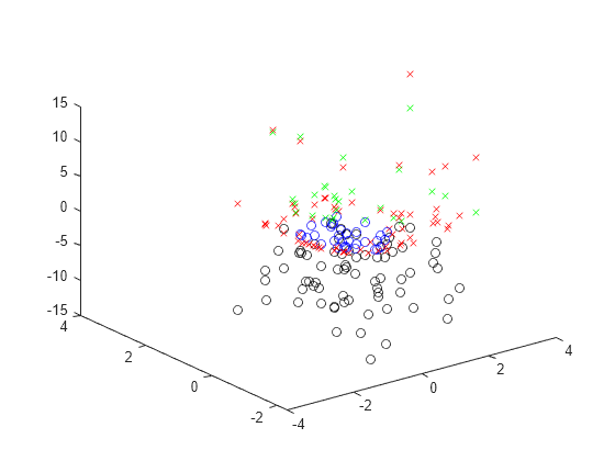
Figure contains an axes object. The axes object contains 4 objects of type line. One or more of the lines displays its values using only markers

As the last figure shows, evaluate enables you to calculate both the value and the feasibility of points. In contrast, issatisfied calculates only the feasibility.

Create a set of equations in two optimization variables.

x = optimvar("x"); y = optimvar("y"); prob = eqnproblem; prob.Equations.eq1 = x^2 + y^2/4 == 2; prob.Equations.eq2 = x^2/4 + 2*y^2 == 2;

Solve the system of equation starting from x=1,y=1/2.

x0.x = 1; x0.y = 1/2; sol = solve(prob,x0)

Solving problem using fsolve.

Equation solved.

fsolve completed because the vector of function values is near zero as measured by the value of the function tolerance, and the problem appears regular as measured by the gradient.

sol = struct with fields: x: 1.3440 y: 0.8799

Evaluate the equations at the points x0 and sol.

vars = optimvalues(prob,x=[x0.x sol.x],y=[x0.y sol.y]); vals = evaluate(prob,vars)

vals = 1×2 OptimizationValues vector with properties:

Variables properties: x: [1 1.3440] y: [0.5000 0.8799]

Equation properties: eq1: [0.9375 8.4322e-10] eq2: [1.2500 6.7431e-09]

The first point, x0, has nonzero values for both equations eq1 and eq2. The second point, sol, has nearly zero values of these equations, as expected for a solution.

Find the degree of equation satisfaction using issatisfied.

[satisfied details] = issatisfied(prob,vars)

satisfied = 1×2 logical array

0 1

details = 1×2 OptimizationValues vector with properties:

Variables properties: x: [1 1.3440] y: [0.5000 0.8799]

Equation properties: eq1: [0 1] eq2: [0 1]

The first point, x0, is not a solution, and satisfied is 0 for that point. The second point, sol, is a solution, and satisfied is 1 for that point. The equation properties show that neither equation is satisfied at the first point, and both are satisfied at the second point.

Input Arguments

collapse all

Optimization expression, specified as an OptimizationExpression object.

Example: expr = 5*x+3, where x is anOptimizationVariable

Values of the variables in an expression, specified as a structure. The structure pt has the following requirements:

All variables in expr must match field names in pt.
The values of the matching field names must be numeric.
The sizes of the fields in pt must match the sizes of the corresponding variables in expr.

For example, pt can be the solution to an optimization problem, as returned by solve.

Example: pt.x = 3, pt.y = -5

Data Types: struct

Constraint, specified as an OptimizationConstraint object, an OptimizationEquality object, or an OptimizationInequality object. evaluate applies to these constraint objects only for a point specified as a structure, not as an OptimizationValues object.

Example: cons = expr1 <= expr2, where expr1 and expr2 are optimization expressions

Object for evaluation, specified as an OptimizationProblem object or an EquationProblem object. The evaluate function evaluates the objectives and constraints in the properties of prob at the points in pts.

Example: prob = optimproblem(Objective=obj,Constraints=constr)

Points to evaluate for prob, specified as a structure or an OptimizationValues object.

The field names in pts must match the corresponding variable names in the objective and constraint expressions inprob.
The values in pts must be numeric arrays of the same size as the corresponding variables in prob.

Note

Currently, pts can be an OptimizationValues object only when prob is an EquationProblem object or an OptimizationProblem object.

If you use a structure for pts, then pts can contain only one point. In other words, if you want to evaluate multiple points simultaneously, pts must be an OptimizationValues object.

Example: pts = optimvalues(prob,x=xval,y=yval)

Output Arguments

collapse all

Evaluation result, returned as a double or an OptimizationValues object.

When the first input argument is an expression or constraint,val is returned as a double array of the same size as the expression or constraint, and contains its numeric values at pt.
When the first input argument is anOptimizationProblem object orEquationProblem object, val is an OptimizationValues object. val contains the values of the objective and constraints or equations inprob evaluated at the points inpts. If pts containsN points, then val has size 1-by-N. For example, ifprob contains a constraintcon of size 2-by-3, andpts is anOptimizationValues object withN = 5 points, then val has size 1-by-5, and val.Constraints.con has size 2-by-3-by-5.

Warning

The problem-based approach does not support complex values in the following: an objective function, nonlinear equalities, and nonlinear inequalities. If a function calculation has a complex value, even as an intermediate value, the final result might be incorrect.

More About

collapse all

For a constraint expression at a point pt:

If the constraint is L <= R, the constraint value isevaluate(L,pt) – evaluate(R,pt).
If the constraint is L >= R, the constraint value isevaluate(R,pt) – evaluate(L,pt).
If the constraint is L == R, the constraint value isabs(evaluate(L,pt) – evaluate(R,pt)).

Generally, a constraint is considered to be satisfied (or feasible) at a point if the constraint value is less than or equal to a tolerance.

Version History

Introduced in R2017b

expand all

The evaluate function now applies to objective and constraint expressions in OptimizationProblem objects. If the evaluation points are passed as an OptimizationValues object, then the function evaluates the expressions at all points in the object. For an example, seeEvaluate Optimization Problem Values.