issatisfied - Constraint satisfaction of an optimization problem at a set of points - MATLAB (original) (raw)
Constraint satisfaction of an optimization problem at a set of points
Since R2024a
Syntax
Description
[allsat](#mw%5F9c56ba19-69e2-4898-b4c9-41347fda4d5a) = issatisfied([prob](#mw%5Ffa89c2fa-b290-47b8-8655-6145973cce78%5Fsep%5Fmw%5F97ec1311-13a3-4b88-889c-fa9152597c41),[pts](#mw%5Ffa89c2fa-b290-47b8-8655-6145973cce78%5Fsep%5Fmw%5Ff575f25a-47c3-4b9a-9ff6-935fc356cf2b)) returns a logical vector whose length is the number of points in pts. An entry in allsat is true if all the constraints inprob are satisfied to within the default tolerance of1e-6 for the corresponding point in pts. Otherwise, the entry is false.
`val` = issatisfied([cons](#mw%5Ffa89c2fa-b290-47b8-8655-6145973cce78%5Fsep%5Fmw%5Fa3dcab01-b74a-493e-8e2d-b960cc26dc1b),[pt](#mw%5Ffa89c2fa-b290-47b8-8655-6145973cce78%5Fsep%5Fmw%5Ff2b0ef39-0511-44a6-943d-b8df4c6a1a7e)) returns a logical value indicating whether the constraint expression cons is satisfied at the point pt.
[allsat](#mw%5F9c56ba19-69e2-4898-b4c9-41347fda4d5a) = issatisfied(___,[tol](#mw%5F85831caf-58df-49b7-90b3-442f68b3c552)), for any previous input arguments, returns true when the constraints at a point are satisfied to within the value tol, and false otherwise.
[[allsat](#mw%5F9c56ba19-69e2-4898-b4c9-41347fda4d5a),[sat](#mw%5F49e4909d-24e5-4d9c-95df-2dd717425019)] = issatisfied(___) also returns an OptimizationValues object sat. This object's Constraints properties are logical indications of the constraint satisfactions for the associated constraints at the corresponding evaluation point.
Examples
Create an optimization problem with several linear and nonlinear constraints.
x = optimvar("x"); y = optimvar("y"); obj = (10*(y - x^2))^2 + (1 - x)^2; cons1 = x^2 + y^2 <= 1; cons2 = x + y >= 0; cons3 = y <= sin(x); cons4 = 2x + 3y <= 2.5; prob = optimproblem(Objective=obj); prob.Constraints.cons1 = cons1; prob.Constraints.cons2 = cons2; prob.Constraints.cons3 = cons3; prob.Constraints.cons4 = cons4;
Create 100 test points randomly.
rng default % For reproducibility xvals = randn(1,100); yvals = randn(1,100);
Convert the points to an OptimizationValues object for the problem, and determine where all the constraints are satisfied among the points.
vals = optimvalues(prob,x=xvals,y=yvals); allsat = issatisfied(prob,vals);
Plot the feasible (satisfied) points with green circles and the infeasible points with red x marks.
xsat = xvals(allsat);
ysat = yvals(allsat);
xnosat = xvals(allsat);
ynosat = yvals(allsat);
plot(xsat,ysat,"go",xnosat,ynosat,"rx")

Create two optimization variables and a 3-by-2 array of inequality constraints.
x = optimvar("x"); y = optimvar("y"); cons = optimconstr(3,2); cons(1,1) = x^2 + y^2/4 <= 2; cons(1,2) = 3x + y <= 4; cons(2,1) = -x - y^3 <= -3; cons(2,2) = 2x^2 + xy + 4y^2 <= 6; cons(3,1) = 2x + 4xy + y^2 <= 5; cons(3,2) = (4 + xy)^2 <= 24;
Check whether all constraints are satisfied at the point x = 1/2, y = -1/2.
pt.x = 1/2; pt.y = -1/2; allsat = issatisfied(cons,pt)
Not all of the constraints are satisfied. Find out which ones are satisfied.
[allsat,sat] = issatisfied(cons,pt)
sat = 3×2 logical array
1 1 0 1 1 1
All but constraint(2,1) are satisfied.
Create an optimization problem with several linear and nonlinear constraints.
x = optimvar("x"); y = optimvar("y"); obj = (10*(y - x^2))^2 + (1 - x)^2; cons1 = x^2 + y^2 <= 1; cons2 = x + y >= 0; cons3 = y <= sin(x); cons4 = 2x + 3y <= 2.5; prob = optimproblem(Objective=obj); prob.Constraints.cons1 = cons1; prob.Constraints.cons2 = cons2; prob.Constraints.cons3 = cons3; prob.Constraints.cons4 = cons4;
Create 100 test points randomly.
rng default % For reproducibility xvals = randn(1,100); yvals = randn(1,100);
Convert the points to an OptimizationValues object for the problem, and determine where all the constraints are satisfied among the points.
vals = optimvalues(prob,x=xvals,y=yvals); allsat = issatisfied(prob,vals);
Plot the feasible (satisfied) points with green circles and the infeasible points with red x marks.
xsat = xvals(allsat);
ysat = yvals(allsat);
xnosat = xvals(allsat);
ynosat = yvals(allsat);
plot(xsat,ysat,"go",xnosat,ynosat,"rx")

Determine which points are feasible with respect to a tolerance of 1 rather than the default 1e-6.
tol = 1; allsat1 = issatisfied(prob,vals,tol);
Plot the feasible (satisfied) points with green circles and the infeasible points with red x marks.
xsat1 = xvals(allsat1);
ysat1 = yvals(allsat1);
xnosat1 = xvals(allsat1);
ynosat1 = yvals(allsat1);
plot(xsat1,ysat1,"go",xnosat1,ynosat1,"rx")

With a looser definition of constraint satisfaction, more points are feasible.
Create an optimization problem with several linear and nonlinear constraints.
x = optimvar("x"); y = optimvar("y"); obj = (10*(y - x^2))^2 + (1 - x)^2; cons1 = x^2 + y^2 <= 1; cons2 = x + y >= 0; cons3 = y <= sin(x); cons4 = 2x + 3y <= 2.5; prob = optimproblem(Objective=obj); prob.Constraints.cons1 = cons1; prob.Constraints.cons2 = cons2; prob.Constraints.cons3 = cons3; prob.Constraints.cons4 = cons4;
Create 100 test points randomly.
rng default % For reproducibility xvals = randn(1,100); yvals = randn(1,100);
Convert the points to an OptimizationValues object for the problem.
vals = optimvalues(prob,x=xvals,y=yvals);
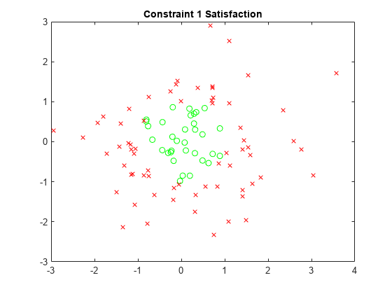
Evaluate the constraints at the points. issatisfied evaluates all the constraint satisfactions at all the test points simultaneously.
[~,sat] = issatisfied(prob,vals);
Plot the feasible (satisfied) points for the first constraint with green circles and the infeasible points with red x marks.
x1sat = xvals(sat.cons1);
y1sat = yvals(sat.cons1);
x1nosat = xvals(sat.cons1);
y1nosat = yvals(sat.cons1);
plot(x1sat,y1sat,"go",x1nosat,y1nosat,"rx")
title("Constraint 1 Satisfaction")
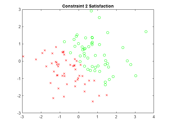
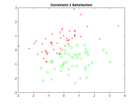
Repeat this process for the other three constraints.
x2sat = xvals(sat.cons2);
y2sat = yvals(sat.cons2);
x2nosat = xvals(sat.cons2);
y2nosat = yvals(sat.cons2);
plot(x2sat,y2sat,"go",x2nosat,y2nosat,"rx")
title("Constraint 2 Satisfaction")
x3sat = xvals(sat.cons3);
y3sat = yvals(sat.cons3);
x3nosat = xvals(sat.cons3);
y3nosat = yvals(sat.cons3);
plot(x3sat,y3sat,"go",x3nosat,y3nosat,"rx")
title("Constraint 3 Satisfaction")
x4sat = xvals(sat.cons4);
y4sat = yvals(sat.cons4);
x4nosat = xvals(sat.cons4);
y4nosat = yvals(sat.cons4);
plot(x4sat,y4sat,"go",x4nosat,y4nosat,"rx")
title("Constraint 4 Satisfaction")

The plots show the different regions of satisfaction for each constraint.
Create a set of equations in two optimization variables.
x = optimvar("x"); y = optimvar("y"); prob = eqnproblem; prob.Equations.eq1 = x^2 + y^2/4 == 2; prob.Equations.eq2 = x^2/4 + 2*y^2 == 2;
Solve the system of equation starting from x=1,y=1/2.
x0.x = 1; x0.y = 1/2; sol = solve(prob,x0)
Solving problem using fsolve.
Equation solved.
fsolve completed because the vector of function values is near zero as measured by the value of the function tolerance, and the problem appears regular as measured by the gradient.
sol = struct with fields: x: 1.3440 y: 0.8799
Evaluate the equations at the points x0 and sol.
vars = optimvalues(prob,x=[x0.x sol.x],y=[x0.y sol.y]); vals = evaluate(prob,vars)
vals = 1×2 OptimizationValues vector with properties:
Variables properties: x: [1 1.3440] y: [0.5000 0.8799]
Equation properties: eq1: [0.9375 8.4322e-10] eq2: [1.2500 6.7431e-09]
The first point, x0, has nonzero values for both equations eq1 and eq2. The second point, sol, has nearly zero values of these equations, as expected for a solution.
Find the degree of equation satisfaction using issatisfied.
[satisfied details] = issatisfied(prob,vars)
satisfied = 1×2 logical array
0 1
details = 1×2 OptimizationValues vector with properties:
Variables properties: x: [1 1.3440] y: [0.5000 0.8799]
Equation properties: eq1: [0 1] eq2: [0 1]
The first point, x0, is not a solution, and satisfied is 0 for that point. The second point, sol, is a solution, and satisfied is 1 for that point. The equation properties show that neither equation is satisfied at the first point, and both are satisfied at the second point.
Input Arguments
Object for evaluation, specified as an OptimizationProblem object or an EquationProblem object. The issatisfied function evaluates the objectives and constraints in the properties of prob at the points in pts.
Example: prob = optimproblem(Objective=obj,Constraints=constr)
Points to evaluate for prob, specified as a structure or an OptimizationValues object.
- The field names in
ptsmust match the corresponding variable names in the objective and constraint expressions inprob. - The values in
ptsmust be numeric arrays of the same size as the corresponding variables inprob.
Note
Currently, pts can be an OptimizationValues object only when prob is an EquationProblem object or an OptimizationProblem object.
If you use a structure for pts, then pts can contain only one point. In other words, if you want to evaluate multiple points simultaneously, pts must be an OptimizationValues object.
Example: pts = optimvalues(prob,x=xval,y=yval)
Constraint, specified as an OptimizationConstraint object, an OptimizationEquality object, or an OptimizationInequality object. issatisfied applies to these constraint objects only for a point specified as a structure, not as an OptimizationValues object.
Example: cons = expr1 <= expr2, where expr1 and expr2 are optimization expressions
Values of the variables in an expression, specified as a structure. The structure pt has the following requirements:
- All variables in
exprmust match field names inpt. - The values of the matching field names must be numeric.
- The sizes of the fields in
ptmust match the sizes of the corresponding variables inexpr.
For example, pt can be the solution to an optimization problem, as returned by solve.
Example: pt.x = 3, pt.y = -5
Data Types: struct
Tolerance for constraint satisfaction, specified as a nonnegative scalar. A constraint is considered to be satisfied if it evaluates to no more thantol. Otherwise, the constraint is unsatisfied.
For example, if c(x) is a nonlinear inequality constraint function, then when c(pt) ≤ tol,issatisfied returns true for that constraint at the point pt. Similarly, if ceq(x) is a nonlinear equality constraint function, then when abs(ceq(pt)) ≤tol, issatisfied returnstrue for that constraint at the point pt.
Data Types: double
Output Arguments
Indication that all constraints are satisfied at the given points, returned as a logical row vector. allsat(i) corresponds to the query pointpts(i). The returned value is true if all values of the constraint functions are no more than tol. Ifpts is a structure, then sat is a logical scalar.
Indication that a constraint is satisfied at the given points, returned as an OptimizationValues vector for an OptimizationProblem or EquationProblem object, or a logical array for a constraint object.
For a problem object, index into sat using the constraint (equation) names. Each entry in sat has the same size as the associated constraint expression.. For example, if pts is anOptimizationValues object with N = 5 points, andcon is a constraint expression of size 2-by-3, thensat.con has size 2-by-3-by-5. The entries aretrue for satisfied constraints to within the tolerancetol.
For a constraint object (OptimizationConstraint, OptimizationEquality, or OptimizationInequality), the size of sat is the same as the size of the associated constraint.
More About
For a constraint expression at a point pt:
- If the constraint is
L <= R, the constraint value isevaluate(L,pt)–evaluate(R,pt). - If the constraint is
L >= R, the constraint value isevaluate(R,pt)–evaluate(L,pt). - If the constraint is
L == R, the constraint value isabs(evaluate(L,pt) – evaluate(R,pt)).
Generally, a constraint is considered to be satisfied (or feasible) at a point if the constraint value is less than or equal to a tolerance.
Version History
Introduced in R2024a
The issatisfied function now applies to objective and constraint expressions in OptimizationProblem objects. If the evaluation points are passed as an OptimizationValues object, then the function determines satisfaction at all points in the object. For an example, see Determine Which Constraints are Satisfied.