Solve Nonlinear Feasibility Problem, Problem-Based - MATLAB & Simulink (original) (raw)
This example shows how to find a point that satisfies all the constraints in a problem, with no objective function to minimize.
Problem Definition
Suppose you have the following constraints:
(y+x2)2+0.1y2≤1y≤exp(-x)-3y≤x-4.
Do any points (x,y) satisfy all of the constraints?
Problem-Based Solution
Create an optimization problem that has only constraints, no objective function.
x = optimvar('x'); y = optimvar('y'); prob = optimproblem; cons1 = (y + x^2)^2 + 0.1*y^2 <= 1; cons2 = y <= exp(-x) - 3; cons3 = y <= x - 4; prob.Constraints.cons1 = cons1; prob.Constraints.cons2 = cons2; prob.Constraints.cons3 = cons3; show(prob)
OptimizationProblem :
Solve for:
   x, y

minimize :

subject to cons1:
   ((y + x.^2).^2 + (0.1 .* y.^2)) <= 1

subject to cons2:
   y <= (exp((-x)) - 3)

subject to cons3:
   y - x <= -4
Create a pseudorandom start point structure x0 with fields x and y for the optimization variables.
rng default x0.x = randn; x0.y = randn;
Solve the problem starting from x0.
[sol,~,exitflag,output] = solve(prob,x0)
Solving problem using fmincon.
Local minimum found that satisfies the constraints.
Optimization completed because the objective function is non-decreasing in feasible directions, to within the value of the optimality tolerance, and constraints are satisfied to within the value of the constraint tolerance.
sol = struct with fields: x: 1.7903 y: -3.0102
exitflag = OptimalSolution
output = struct with fields: iterations: 6 funcCount: 9 constrviolation: 0 stepsize: 0.2906 algorithm: 'interior-point' firstorderopt: 0 cgiterations: 0 message: 'Local minimum found that satisfies the constraints.↵↵Optimization completed because the objective function is non-decreasing in ↵feasible directions, to within the value of the optimality tolerance,↵and constraints are satisfied to within the value of the constraint tolerance.↵↵↵↵Optimization completed: The relative first-order optimality measure, 0.000000e+00,↵is less than options.OptimalityTolerance = 1.000000e-06, and the relative maximum constraint↵violation, 0.000000e+00, is less than options.ConstraintTolerance = 1.000000e-06.' bestfeasible: [1×1 struct] objectivederivative: "closed-form" constraintderivative: "forward-AD" solver: 'fmincon'
The solver finds a feasible point.
Importance of Initial Point
The solver can fail to find a solution when starting from some initial points. Set the initial point x0.x = –1, x0.y = –4 and then solve the problem starting from x0.
x0.x = -1; x0.y = -4; [sol2,~,exitflag2,output2] = solve(prob,x0)
Solving problem using fmincon.
Converged to an infeasible point.
fmincon stopped because the size of the current step is less than the value of the step size tolerance but constraints are not satisfied to within the value of the constraint tolerance.
Consider enabling the interior point method feasibility mode.
sol2 = struct with fields: x: -2.1266 y: -4.6657
exitflag2 = NoFeasiblePointFound
output2 = struct with fields: iterations: 129 funcCount: 283 constrviolation: 1.4609 stepsize: 1.3726e-10 algorithm: 'interior-point' firstorderopt: 0 cgiterations: 265 message: 'Converged to an infeasible point.↵↵fmincon stopped because the size of the current step is less than↵the value of the step size tolerance but constraints are not↵satisfied to within the value of the constraint tolerance.↵↵↵↵Optimization stopped because the relative changes in all elements of x are↵less than options.StepTolerance = 1.000000e-10, but the relative maximum constraint↵violation, 1.521734e-01, exceeds options.ConstraintTolerance = 1.000000e-06.' bestfeasible: [] objectivederivative: "closed-form" constraintderivative: "forward-AD" solver: 'fmincon'
Check the infeasibilities at the returned point.
inf1 = infeasibility(cons1,sol2)
inf2 = infeasibility(cons2,sol2)
inf3 = infeasibility(cons3,sol2)
Both cons1 and cons3 are infeasible at the solution sol2. The results highlight the importance of using multiple start points to investigate and solve a feasibility problem.
Visualize Constraints
To visualize the constraints, plot the points where each constraint function is zero by using fimplicit. The fimplicit function passes numeric values to its functions, whereas the evaluate function requires a structure. To tie these functions together, use the evaluateExpr helper function, which appears at the end of this example. This function simply puts passed values into a structure with the appropriate names.
Note: Make sure the code for the evaluateExpr helper function is included at the end of your script or in a file on the path.
Avoid a warning that occurs because the evaluateExpr function does not work on vectorized inputs.
s = warning('off','MATLAB:fplot:NotVectorized'); cc1 = (y + x^2)^2 + 0.1*y^2 - 1; fimplicit(@(a,b)evaluateExpr(cc1,a,b),[-2 2 -4 2],'r') hold on cc2 = y - exp(-x) + 3; fimplicit(@(a,b)evaluateExpr(cc2,a,b),[-2 2 -4 2],'k') cc3 = y - x + 4; fimplicit(@(x,y)evaluateExpr(cc3,x,y),[-2 2 -4 2],'b') hold off
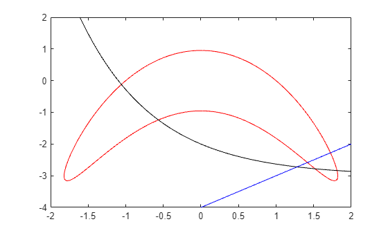
The feasible region is inside the red outline and below the black and blue lines. The feasible region is at the lower right of the red outline.
Helper Function
This code creates the evaluateExpr helper function.
function p = evaluateExpr(expr,x,y) pt.x = x; pt.y = y; p = evaluate(expr,pt); end