Monitor Pool Workers with Pool Dashboard - MATLAB & Simulink (original) (raw)
Pool monitoring data helps you understand how pool workers execute parallel constructs like parfor, parfeval, andspmd on parallel pools. The Pool Dashboard collects monitoring data, including information about how workers execute your parallel code and the data transfers involved. This information helps you identify bottlenecks, balance workloads, and ensure efficient resource utilization and optimize the performance of your parallel code.
You can collect pool activity monitoring data interactively with the Pool Dashboard or programmatically using an ActivityMonitor object and view the data in the Pool Dashboard. For most use cases, use thePool Dashboard to interactively collect and view monitoring data. However, if you need to collect monitoring data to review later or for code that runs on a batch parallel pool, use the ActivityMonitor object. For details, seeProgrammatically Collect Pool Monitoring Data.
To open the Pool Dashboard, select one of these options:
- MATLAB® Toolstrip: On the tab, in the section, select > .
- Parallel status indicator: Click the indicator icon and select .
- MATLAB command prompt: Enter
parpoolDashboard.
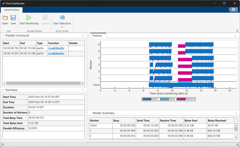
The Pool Dashboard displays monitoring data in these sections.
| Section | Details |
|---|---|
| Parallel Constructs | Displays information about the types of parallel constructs the workers execute, the parent function or script that calls the parallel construct, and details of the functions the parallel constructs run, if available. |
| Timeline | Provides a visual representation of the time workers and the client spend running the parallel construct and transferring data. For example, dark blue represents time spent running aparfor-loop, light blue represents time spent sending data, and magenta represents time spent receiving data. When you select a specific parallel construct, elements in the Timeline graph unrelated to the selected construct appear in gray.The Timeline graph can only display pool monitoring data for up to 32 workers. |
| Summary | Summarizes the entire monitoring session, including the start and stop monitoring times, total busy time, bytes of data the client sends to the workers, and parallel efficiency, which is the percentage of time the workers are busy relative to the monitored time. |
| Worker Summary | Condenses the information from the Timeline graph, providing an overview of each worker's activity. |
| Call Stack | Expands on the information about the parent function or script that calls the parallel construct and the functions the parallel construct runs. The Call Stack is only visible when you select a specific parallel construct. |
Use these examples to explore the features of the Pool Dashboard.
Compare Performance of Parallel Code
This example shows how to use the Pool Dashboard to compare the performance of parfor-loops.
When you initialize a variable before a parfor-loop and use it inside the loop, you must pass it to each MATLAB® worker evaluating the loop iterations. The parfor function transfers only the variables that the loop uses from the client workspace to the workers. However, if the loop variable indexes all occurrences of the variable, parfor slices the variable and sends each worker only the part of the variable it needs. Using sliced variables reduces data transfer overheads between the client and workers.
Compare the performance of a parfor-loop with sliced variables to one without sliced variables by collecting monitoring data with the Pool Dashboard.
Open the Pool Dashboard. In the Monitoring section of the Pool Dashboard, click Start Monitoring. When the Pool Dashboard begins collecting monitoring data, return to the Live Editor and click Run Section.

In this code, parfor breaks the data variable into slices, which are then operated on separately by different workers.
A = 500; M = 100; N = 1e6; data = randn(M,N); parfor idx = 1:M a = max(abs(eig(rand(A)))); b = sum(data(idx, :))./N; r(idx) = a*b; end pause(1)
Now, suppose that you accidentally use a reference to the data variable instead of N inside the parfor-loop. The problem is that the call to size(data,2) converts the sliced variable data into a broadcast (non-sliced) variable.
parfor idx = 1:M a = max(abs(eig(rand(A)))); b = sum(data(idx,:))./size(data,2); r(idx) = a*b; end
disp("Section complete!")
After the section code is complete, in the Monitoring section , select Stop. The Pool Dashboard displays the monitoring results.
The Pool Dashboard displays information for both parfor-loops, separated by the one second pause.
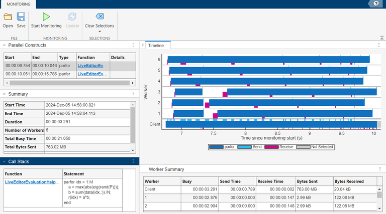
In the Parallel Constructs table, select the first parfor computation, which is the parfor-loop with the sliced data variable. The Timeline graph and the Summary and Worker Summary tables now display information specific to the selected parfor-loop. Elements in the Timeline graph unrelated to the selected construct appear in gray. The Call Stack table is now visible below the Summary table. To expand the Call Stack table, click the right arrow. The Call Stack table displays the parfor-loop in the Statement column.
The Timeline graph indicates that each worker takes a similar amount of time to execute their parfor iterations and the workers are not idle for long. Data transfer durations are also brief. In the Summary table, note the parfor-loop execution duration of 3.291 seconds and the data the client sends to the workers, totaling 763.02 MB.
In the Parallel Constructs table, select the second parfor construct, which is the parfor-loop with the accidentally broadcast data variable. The Timeline graph indicates the workers spend the first one to two seconds receiving data from the client. In the Summary table, the parfor-loop execution duration is 5.734 seconds and the client sends a total of 763.02 MB of data to the workers. The execution duration is greater for the parfor-loop with the accidentally broadcast variable due to the large data being transferred to the workers.
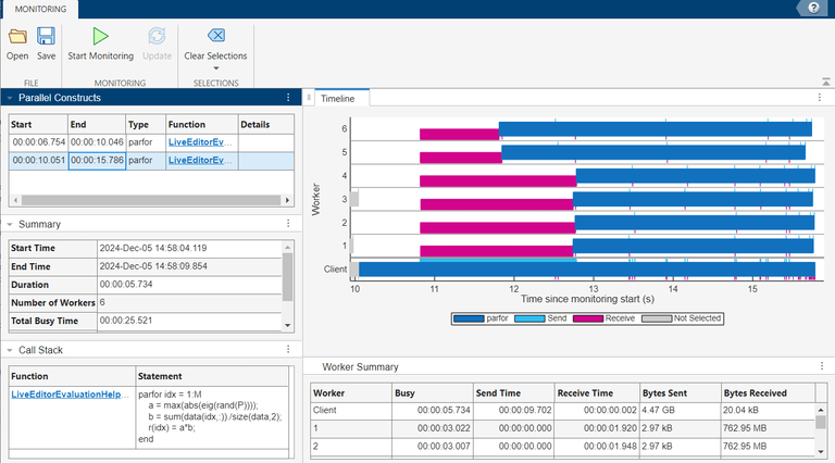
As the result is a constant, you can avoid the non-sliced usage of the data variable by computing it outside the loop. Generally, perform computations that depend solely on broadcast data before the loop starts, because broadcast data cannot be modified inside the loop. In this case, the computation is trivial, and results in a scalar, so you benefit from taking the computation out of the loop.
Identify parfeval Computations in Monitoring Data
This example shows how to identify details of parfeval computations in monitoring data the Pool Dashboard displays.
The parfeval function performs asynchronous execution of functions on workers without blocking the client. Workers execute the function at any time, which makes it challenging to determine when execution completes. When you collect pool monitoring data for parfeval computations, the Pool Dashboard displays this data in a way that enables you to identify the details of a specific parfeval computation among similar computations.
Start a pool of three workers.
Starting parallel pool (parpool) using the 'Processes' profile ... Connected to parallel pool with 3 workers.
Collect pool monitoring data for a set of parfeval computations, each running a different function.
Open the Pool Dashboard. In the Monitoring section of the Pool Dashboard, select Start Monitoring. When the Pool Dashboard begins collecting monitoring data, return to the Live Editor and select Run Section.

Execute the dollarAuctionModels helper function, attached to this example as a supporting file. The dollarAuctionModels function runs Monte-Carlo simulations of different dollar auction models with a specified number of trials asynchronously using the parfeval function.
numTrials = 1000; auctionFutures = dollarAuctionModels(1000);
Introduce a short pause to simulate a delay between scheduling parfeval computations.
Execute a series of asynchronous parfeval computations to price financial options using Monte-Carlo methods. The helper functions for these models are also attached to this example as supporting files.
Define a list of models to run.
modelFunctions = {@mcAsianCallOption,@mcDownAndOutCallOption,@mcLookbackCallOption,@mcStockPrice,@mcUpAndOutCallOption}; numModels = length(modelFunctions);
Load input parameters for the models.
Use parfeval to simulate each model in parallel.
optionFutures(1:numModels) = parallel.FevalFuture; for m = 1:numModels optionFutures(m) = parfeval(modelFunctions{m},1,params); end
Use parfevalOnAll to execute a brief pause on all workers to ensure all the parfeval computations are completed before you stop collecting pool monitoring data.
syncF = parfevalOnAll(@pause,0,0.1); wait(syncF)
disp("Section complete.")
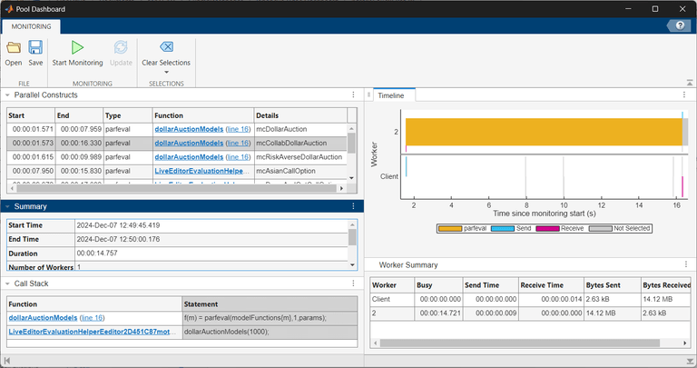
After the section code is complete, in the Monitoring section of the Pool Dashboard, select Stop. The Pool Dashboard displays the monitoring results.
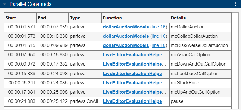
Unlike the results from monitoring a parfor-loop, the Parallel Constructs table lists the name of the function that each parfeval computation evaluates in the Details column. The Function column lists the parent function or script that schedules the parfeval computation. For example, the dollarAuctionModels function uses the parfeval function to evaluate the mcDollarAuction, mcCollabDollarAuction, and mcRiskAverseDollarAuction helper functions.
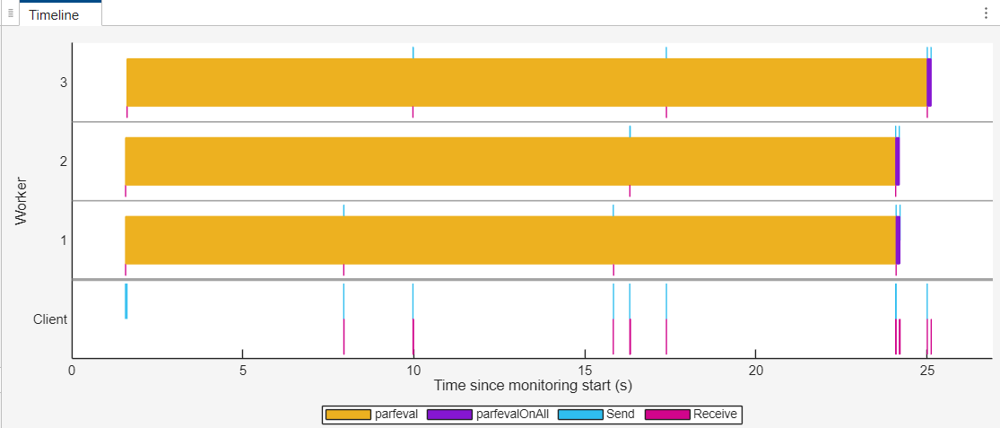
The Timeline graph represents the time workers spend running parfeval computations in yellow and parfevalOnAll computations in purple. The same parfevalOnAll computation occurs on all the workers at different times. You can observe that each worker completes multiple parfeval computations with no idle time between them. The data transfer bars in blue and magenta help differentiate the various parfeval bars. The first parfeval bar on worker 2 is longer than the others. To identify the code responsible for the long-running parfeval computation, select that bar.
The Timeline graph and the Summary and Worker Summary tables now display information specific to the selected parfeval computation, and the Parallel Constructs table highlights the row for the selected parfeval bar. The Call Stack table for the selected parfeval computation is now visible below the Summary table. To expand the Call Stack table, click the right arrow. The Call Stack table shows the parfeval function call in the Statement column. This information indicates that the Live Editor script calls the dollarAuctionModels function, which in turn schedules the long-running parfeval computation. The parfeval computation evaluates the mcCollabDollarAuction function.
To clear the information for the currently selected parfeval computation and view activity data for all the workers again, in the Selections section of the Pool Dashboard, click Clear Selections.
Analyze Distributed Array Computations
This example shows how to analyze pool monitoring data you collect during computations with distributed arrays.
A distributed array is a single variable, divided over multiple workers in your parallel pool. When you apply functions to distributed arrays, MATLAB® uses spmd statements to execute these functions simultaneously on all the workers of the pool. The Pool Dashboard collects monitoring data for each spmd computation.
In this example, you collect and analyze pool monitoring data while solving a system of linear equations with distributed arrays on a parallel pool of cluster workers.
Start a parallel pool of cluster workers using the remote cluster profile MyCluster.
pool = parpool("MyCluster",12);
Starting parallel pool (parpool) using the 'MyCluster' profile ... Connected to parallel pool with 12 workers.
Open the Pool Dashboard. In the Monitoring section of the Pool Dashboard, click Start Monitoring. When the Pool Dashboard begins collecting monitoring data, return to the Live Editor and click Run Section.

Define the size of a suitably large array for the number of workers in the pool.
nWorkers = pool.NumWorkers; n = floor(sqrt(40964096nWorkers));
To directly construct distributed arrays on the workers, use the "distributed" argument of the randi and ones functions. Define the coefficient matrix A and the exact solutions for comparison, xEx.
A = randi(100,n,n,"distributed"); xEx = ones(n,1,"distributed");
Define the right-hand vector b as the row sum of A. The vector b is also distributed.
Use mldivide to solve the system directly.
Calculate the mean error between each element of the obtained result x and the expected values of xEx.
err = abs(xEx-x); mErr = mean(err);
disp("Section complete.")
After the section code is complete, in the Monitoring section of the Pool Dashboard, select Stop. The Pool Dashboard displays the monitoring results.
The Parallel Constructs table and Timeline graph display computations on distributed arrays as spmd computations. The count of spmd computations in the Parallel Constructs table and Timeline graph corresponds to the frequency with which MathWorks® utility functions invoke spmd to execute code on the distributed arrays.
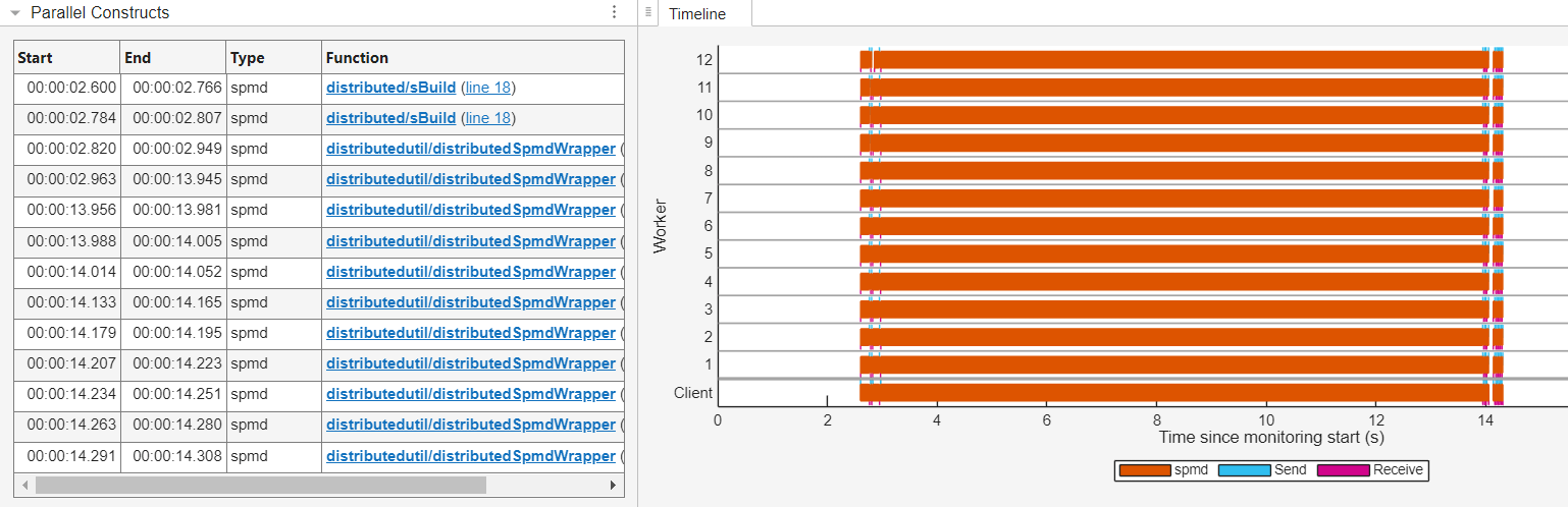
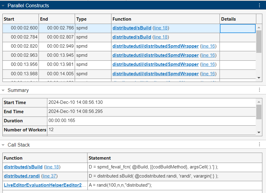
The Parallel Constructs table lists the utility functions that call spmd in the Function column. You can identify the line of code responsible for any spmd computation in the Call Stack table. For example, to view the Call Stack table for the spmd computation initiated by the utility function distributed/sBuild, select the first row in the Parallel Constructs table. The Call Stack table for the selected spmd computation is now visible below the Summary table. To expand the Call Stack table, click the right arrow.
The Call Stack table provides detailed information about the code responsible for the spmd computation in hierarchical order, with the parent function or script and specific code line appearing in the bottom row. The information in the Call Stack table indicates the utility function distributed/sBuild creates the distributed array A on the workers.
To clear the information for the currently selected spmd computation and view monitoring data for all spmd computations again, in the Selections section of the Pool Dashboard, click Clear Selections.
The Timeline graph visually represents the duration of the spmd computations on each worker as orange bars. The data send and receive bars in blue and magenta help differentiate the various spmd bars. Look for the longest orange bar on any worker, which indicates the longest-running spmd computation. Select the bar.
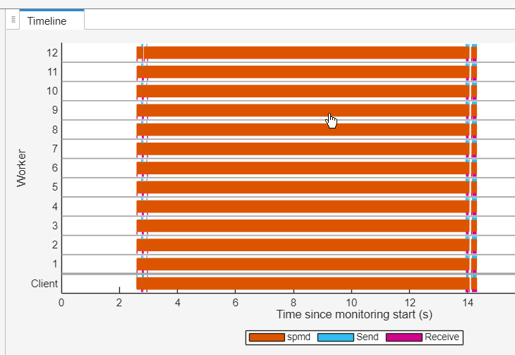
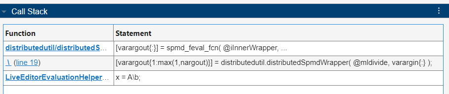
The Timeline graph, Summary, and Worker Summary tables now display information specific to the selected spmd computation, and the Parallel Constructs table highlights the row for the selected spmd bar. The Call Stack table for the selected spmd computation is also visible. The Call Stack information indicates that the longest-running spmd statement evaluates the mldivide function.
Measure and Improve Parallel Efficiency
This example shows how to use the Pool Dashboard to measure and improve the parallel efficiency of computations on a parallel pool.
The Pool Dashboard parallel efficiency metric helps you identify inefficiencies in your parallel pool workflow. The Pool Dashboard calculates parallel efficiency using the formula:
Parallel Efficiency=(Total Busy TimeNumber of Workers x Duration) x 100,
where
- Total Busy Time is the cumulative time all workers actively process tasks.
- Duration is the total time from start to end of the monitoring period.
- Number of Workers is the total number of workers in the parallel pool.
In this example, you collect pool monitoring data while executing a workflow to import and automatically process data using an interactive parallel pool. Use the pool monitoring data, particularly the parallel efficiency metric, to determine if the workflow uses the pool workers efficiently.
Measure Parallel Efficiency
Start a parallel pool of six workers.
Starting parallel pool (parpool) using the 'Processes' profile ... Connected to parallel pool with 6 workers.
Open the Pool Dashboard. In the Monitoring section of the Pool Dashboard, click Start Monitoring. When the Pool Dashboard begins collecting monitoring data, return to the Live Editor and click Run Section.

Acquire and automatically process data iteratively. Schedule the importDataFromDatabase function to import data asynchronously with parfeval, then process the data using the processData function in a parfor-loop. The importDataFromDatabase and processData helper functions are defined at the end of this example.
numIter = 3; w = 30; for idx = 1:numIter future = parfeval(@importDataFromDatabase,1,w); data = fetchOutputs(future); parfor col = 1:w out(col) = processData(data(:,col)); end end
disp("Section complete.")
After the section code is complete, in the Monitoring section of the Pool Dashboard, select Stop. The Pool Dashboard displays the monitoring results.
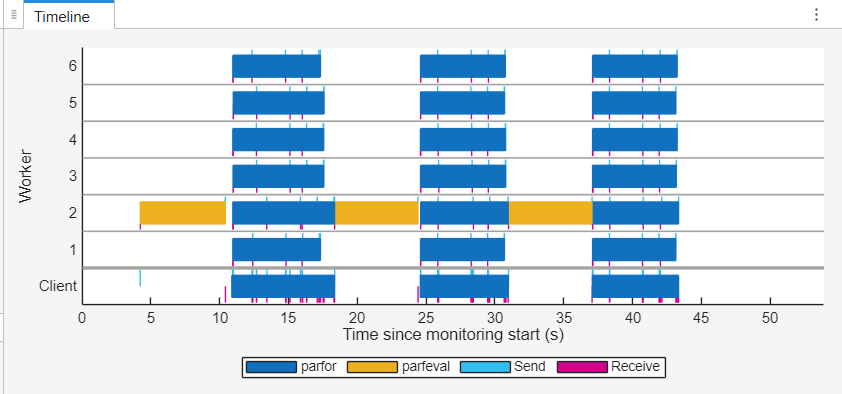
The Timeline graph indicates that most of the workers remain idle during the parfeval execution. This idle time stems from the code structure, where the parfor-loop cannot begin until the parfeval computation is complete.
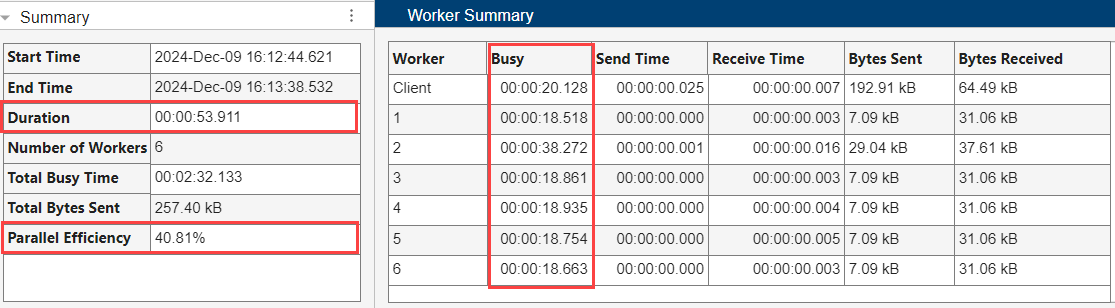
In the Worker Summary table, the maximum busy time of the workers is 38.272 seconds out of a total duration of 53.911 seconds. The parallel efficiency for the workflow is 40.81%, indicating that the workers are not being used effectively.
The pool monitoring data highlights inefficiencies in the parallel processing code. The code uses asynchronous parfeval computations to import data and then waits for the computations to complete before proceeding with a parfor-loop to process the data. This approach introduces unnecessary delays, as the loop waits for the parfeval computation sequentially, which prevents the software from fully using the parallel workers.
Improve Parallel Efficiency
To enhance parallel efficiency, restructure the code to overlap data import and processing tasks, minimizing worker idle time. Initiate the first data import asynchronously before you start the for-loop. This restructure allows the workers to continue executing other tasks while waiting for the data import to complete.
Run the restructured code and collect monitoring data with the Pool Dashboard. In the Monitoring section of the Pool Dashboard, click Start Monitoring. When the Pool Dashboard begins collecting monitoring data, return to the Live Editor and click Run Section.
 future = parfeval(@importDataFromDatabase,1,w);
for idx = 1:numIter data = fetchOutputs(future); if idx < numIter future = parfeval(@importDataFromDatabase,1,w); end parfor col = 1:w out(col) = processData(data(:,col)); end end
disp("Section complete.")
After the section code is complete, in the Monitoring section of the Pool Dashboard, select Stop. The Pool Dashboard displays the monitoring results.
The Timeline graph displays the overlap between data import parfeval and data processing parfor computations. The parfeval computations now occur asynchronously and the parfor-loop does not wait for the parfeval computations to complete before executing with the remaining workers of the pool.
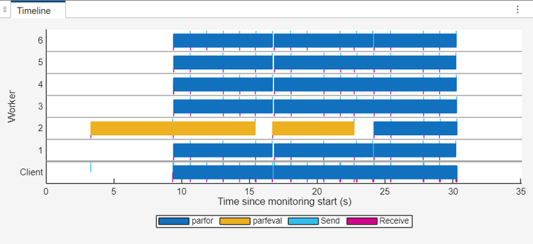
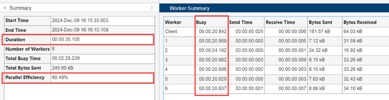
The Worker Summary table still shows similar worker busy times when compared to the inefficient parallel code, however, the workflow duration is decreased to 35 seconds. This shorter duration results in an increase in the parallel efficiency for the workflow from 40.81% to 60.48%.
Helper Functions
The importDataFromDatabase function simulates the import of data from a database. The function generates a magic square matrix of size specified by the input in and simulates a delay by pausing for 6 seconds.
function out = importDataFromDatabase(in) out = magic(in); pause(6) end
The processData function calculates the sum of the elements in the input data and simulates a nontrivial calculation by pausing for 1.2 seconds.
function out = processData(data) out = sum(data); pause(1.2) end
See Also
Functions
- parfor | parfeval | distributed | spmd