Try Parallel Computing Methods - MATLAB & Simulink (original) (raw)

This example shows how to accelerate your MATLAB® code using parallel computing. Try the example to see how to begin using parallel computing in MATLAB.

This graph shows the execution times for three parallel computing methods compared to serial computing when running the algorithm used in this example. Your results will depend on your hardware.

Bar graph showing the execution times for three parallel computing methods compared to serial computing when running the algorithm used in this example.

Develop Algorithm

Start by prototyping your algorithm. In this example, you use the computePi function to run a Monte Carlo algorithm that estimates the value of π.

The algorithm performs these steps:

Randomly generate m sets of x- and y-coordinates in the range [0,1].
Determine whether the coordinates describe a point inside a circle inscribed within a unit square.
Repeat steps 1 and 2, n times.
Use the number of points in the circle and the total number of points to calculate an estimate of π.

For more details estimating π using a Monte Carlo algorithm, see the Simple Monte Carlo Area Method section.

Create the Monte Carlo algorithm.

function piEst = computePi(m,n) pointsInCircle = 0;

for i = 1:n % Generate random points. x = rand(m,1); y = rand(m,1);

% Determine whether the points lie inside the unit circle.
r = x.^2 + y.^2;
pointsInCircle = pointsInCircle + sum(r<=1);

end

piEst = 4/(m*n) * pointsInCircle; end

Check whether the algorithm computes a reasonable estimate.

m = 3e5; n = 1e3;

piEst = computePi(m,n)

Use the timeit function to measure the time required to run the computePi function.

timeSerial = timeit(@() computePi(m,n))

Experiment with Parallel Processing Methods

You can accelerate this algorithm using parallel processing. In this section, you make minor changes to the code to make it run using three parallel computing methods. You then assess which parallel processing method is most suitable for accelerating the algorithm.

Parfor Method

If your algorithm contains a for-loop and the order of the iterations is not relevant, then converting the for-loop to a parfor-loop is usually the easiest way to parallelize your code.

Define a new function, computePiParfor, that estimates π using a parfor-loop instead of a for-loop.

function piEst = computePiParfor(m,n) pontsInCircle = 0;

parfor i = 1:n % Generate random points. x = rand(m,1); y = rand(m,1);

% Determine whether the points lie inside the unit circle.
r = x.^2 + y.^2;
pontsInCircle = pontsInCircle + sum(r<=1);

end

piEst = 4/(m*n) * pontsInCircle; end

Start a thread-based parallel pool. By default, MATLAB starts a pool with one worker per physical core on your local machine.

pool = parpool("Threads");

Starting parallel pool (parpool) using the 'Threads' profile ... Connected to parallel pool with 6 workers.

Measure the time required to run the computePiParfor function.

timeParfor = timeit(@() computePiParfor(m,n))

Using a parfor-loop significantly accelerates the algorithm with minimal changes to the code.

Parfeval Method

You can use parfeval to run a function on a parallel worker.

Define a function, calculatePoints, that generates m random points and determines whether the points are inside the unit circle. This function corresponds to a single iteration of the for-loop in the original computePi function.

function pointsInCircle = calculatePoints(m) % Generate random points. x = rand(m,1); y = rand(m,1);

% Determine whether the points lie inside the unit circle. r = x.^2 + y.^2; pointsInCircle = sum(r<=1); end

Define a function, computePiParfeval, that estimates π using parfeval. This function calls parfeval in a for-loop to execute the calculatePoints function n times on the workers in the parallel pool. The function then uses the results to generate an estimate of π. Each worker has an independent random number stream, so calls to rand produce a unique sequence of random numbers on each worker. For more information about controlling random number generation on workers, see Control Random Number Streams on Workers.

function piEst = computePiParfeval(m,n)

for i = 1:n f(i) = parfeval(@calculatePoints,1,m); end

output = fetchOutputs(f); piEst = 4/(m*n) * sum(output); end

Measure the time required to run the computePiParfeval function.

timeParfeval = timeit(@() computePiParfeval(m,n))

As you can see from the timing, parfeval is not well-suited to this problem as it is currently formulated because the calculatePoints function runs too quickly, resulting in significant communication and scheduling overheads. However, parfeval is well-suited for problems with a known desired result but for which it is unknown how many iterations it might take to achieve the result. For example, if you want to iteratively refine an estimate of πuntil the solution stops improving, you could use parfeval to queue 10,000 iterations and, when the goal is reached, you can cancel all the remaining iterations. An improved function that calculates π using parfeval, computePiParfevalImproved, is attached to this example as a supporting file. Open this example as a live script to access the supporting file.

GPU Method

If you have a supported GPU, you can accelerate your code by running it on the GPU. For more information about supported GPUs, see GPU Computing Requirements.

gpu = gpuDevice; disp(gpu.Name + " GPU selected.")

NVIDIA RTX A5000 GPU selected.

Define a new function, computePiGPU, that estimates π on a GPU. Many functions in MATLAB and other toolboxes run automatically on a GPU if you supply a gpuArray data argument. The computePiGPU function generates the random points as gpuArray data, and then subsequent calculations are performed on the GPU automatically.

function piEst = computePiGPU(m,n) c = zeros(1,"gpuArray");

for i = 1:n % Generate random points on the GPU. x = rand(m,1,"gpuArray"); y = rand(m,1,"gpuArray");

% Determine whether the points lie inside the unit circle.
r = x.^2 + y.^2;
c = c + sum(r<=1);

end

piEst = 4/(m*n) * c; end

Use the gputimeit function to measure the time required to run the computePiGPU function. The gputimeit function is preferable to timeit for functions that use the GPU, because it ensures that all operations on the GPU have finished before recording the time and it compensates for the overhead.

timeGPU = gputimeit(@() computePiGPU(m,n))

You can further accelerate this code on a GPU by vectorizing the for-loop. Vectorization is the process of revising loop-based code to use MATLAB matrix and vector operations. Vectorizing code is particularly effective in accelerated code that runs on a GPU, as GPUs are generally more effective when performing a large numberof operations. An improved function that calculates π on a GPU using vectorized code, computePiGPUVectorized, is attached to this example as a supporting file. Open this example as a live script to access the supporting file.

Compare Execution Times

Compare the execution times of the parallel methods to the serial execution.

figure bar([timeSerial timeParfor timeParfeval timeGPU]) xlabel("Execution Type") xticklabels(["Serial" "Parfor" "Parfeval" "GPU"]) ylabel("Execution Time (s)") grid on

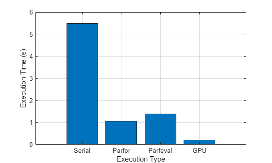
The execution times for the three parallel computing methods are significantly faster compared to serial computing when running the algorithm used in this example. Your results will depend on your hardware.

Simple Monte Carlo Area Method

Given a circle with radius r inscribed within a square with sides of length 2r_,_ the area of the circle is related to the area of the square by π. This figure illustrates the problem.

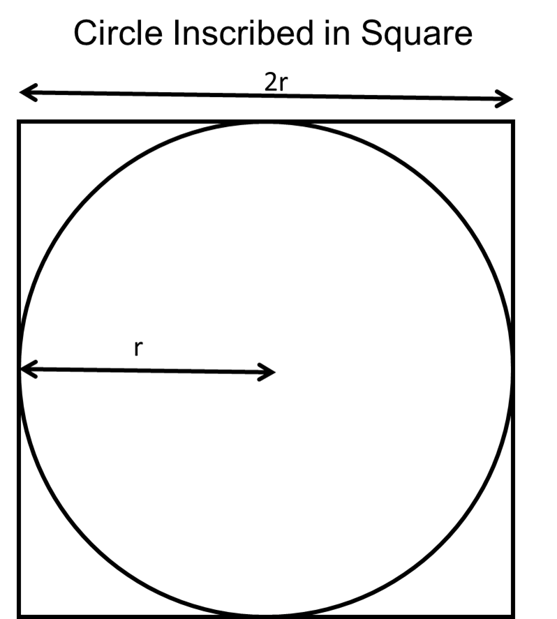
You can derive π from the ratio of the area of the circle divided by the area of the square:

area of circlearea of square=

πr2(2r)2= π4

To estimate the area of the circle without using π directly, randomly generate a uniform sample of points inside the square and count how many of the points are inside the circle. The probability that a point can be found in the circle is the ratio of the area of the circle divided by the area of the square.

To determine whether a point is inside the circle, randomly generate two values for the x- and y-coordinates of a point and calculate the distance between the point and the origin of the circle. The distance d from the origin to the generated point is given by this equation:

d= x2+y2

If d is less than the radius r of the circle, the point is inside the circle. Generate a large sample of points and count how many are inside the circle. Use this data to obtain a ratio of points inside the circle to the total number of points generated. This ratio is equivalent to the ratio of the area of the circle to the area of the square. You can then estimate π using:

points in circletotal number of points≈π4

π≈4×points in circletotal number of points