chirp - Swept-frequency cosine - MATLAB (original) (raw)

Syntax

Description

[y](#d126e19967) = chirp([t](#d126e19576),[f0](#d126e19622),[t1](#d126e19649),[f1](#d126e19676)) generates samples of a linear swept-frequency cosine signal at the time instances defined in array t. The instantaneous frequency at time 0 is f0 and the instantaneous frequency at timet1 is f1.

example

[y](#d126e19967) = chirp([t](#d126e19576),[f0](#d126e19622),[t1](#d126e19649),[f1](#d126e19676),[method](#d126e19708)) specifies an alternative sweep method option.

example

[y](#d126e19967) = chirp([t](#d126e19576),[f0](#d126e19622),[t1](#d126e19649),[f1](#d126e19676),[method](#d126e19708),[phi](#d126e19843)) specifies the initial phase.

example

[y](#d126e19967) = chirp([t](#d126e19576),[f0](#d126e19622),[t1](#d126e19649),[f1](#d126e19676),"quadratic",[phi](#d126e19843),[shape](#d126e19870)) specifies the shape of the spectrogram of a quadratic swept-frequency signal.

example

[y](#d126e19967) = chirp(___,[cplx](#mw%5F810e1e71-270a-491a-8ab5-acc48938487f)) returns a real chirp if cplx is specified as"real" and returns a complex chirp ifcplx is specified as"complex".

example

Examples

collapse all

Generate a chirp with linear instantaneous frequency deviation. The chirp is sampled at 1 kHz for 2 seconds. The instantaneous frequency is 0 at t = 0 and crosses 250 Hz at t = 1 second.

t = 0:1/1e3:2; y = chirp(t,0,1,250);

Compute and plot the spectrogram of the chirp. Divide the signal into segments such that the time resolution is 0.1 second. Specify 99% of overlap between adjoining segments and a spectral leakage of 0.85.

pspectrum(y,1e3,"spectrogram",TimeResolution=0.1, ... OverlapPercent=99,Leakage=0.85)

Generate a chirp with quadratic instantaneous frequency deviation. The chirp is sampled at 1 kHz for 2 seconds. The instantaneous frequency is 100 Hz at t = 0 and crosses 200 Hz at t = 1 second.

t = 0:1/1e3:2; y = chirp(t,100,1,200,"quadratic");

Compute and plot the spectrogram of the chirp. Divide the signal into segments such that the time resolution is 0.1 second. Specify 99% of overlap between adjoining segments and a spectral leakage of 0.85.

pspectrum(y,1e3,"spectrogram",TimeResolution=0.1, ... OverlapPercent=99,Leakage=0.85)

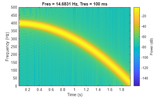
Generate a convex quadratic chirp sampled at 1 kHz for 2 seconds. The instantaneous frequency is 400 Hz at t = 0 and crosses 300 Hz at t = 1 second.

t = 0:1/1e3:2; fo = 400; f1 = 300; y = chirp(t,fo,1,f1,"quadratic",[],"convex");

Compute and plot the spectrogram of the chirp. Divide the signal into segments such that the time resolution is 0.1 second. Specify 99% of overlap between adjoining segments and a spectral leakage of 0.85.

pspectrum(y,1e3,"spectrogram",TimeResolution=0.1, ... OverlapPercent=99,Leakage=0.85)

Generate a concave quadratic chirp sampled at 1 kHz for 4 seconds. Specify the time vector so that the instantaneous frequency is symmetric about the halfway point of the sampling interval, with a minimum frequency of 100 Hz and a maximum frequency of 500 Hz.

t = -2:1/1e3:2; fo = 100; t1 = max(t); f1 = 500; y = chirp(t,fo,t1,f1,"quadratic",[],"concave");

Compute and plot the spectrogram of the chirp. Divide the signal into segments such that the time resolution is 0.1 second. Specify 99% of overlap between adjoining segments and a spectral leakage of 0.85.

pspectrum(y,t,"spectrogram",TimeResolution=0.1, ... OverlapPercent=99,Leakage=0.85)

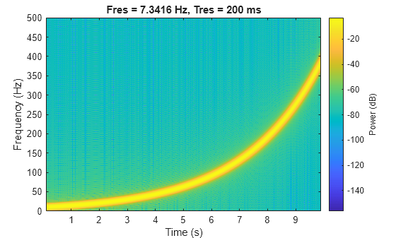
Generate a logarithmic chirp sampled at 1 kHz for 10 seconds. The instantaneous frequency is 10 Hz initially and 400 Hz at the end.

t = 0:1/1e3:10; fo = 10; f1 = 400; y = chirp(t,fo,10,f1,"logarithmic");

Compute and plot the spectrogram of the chirp. Divide the signal into segments such that the time resolution is 0.2 second. Specify 99% of overlap between adjoining segments and a spectral leakage of 0.85.

pspectrum(y,t,"spectrogram",TimeResolution=0.2, ... OverlapPercent=99,Leakage=0.85)

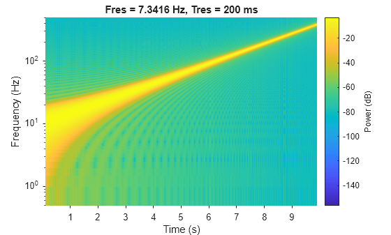
Use a logarithmic scale for the frequency axis. The spectrogram becomes a line, with high uncertainty at low frequencies.

ax = gca; ax.YScale = "log";

Generate a complex linear chirp sampled at 1 kHz for 10 seconds using single support precision. The instantaneous frequency is –200 Hz initially and 300 Hz at the end. The initial phase is zero.

fs = 1e3; t = single(0:1/fs:10); fo = -200; f1 = 300; ph0 = 0;

y = chirp(t,fo,t(end),f1,"linear",ph0,"complex");

Compute and plot the spectrogram of the chirp. Divide the signal into segments such that the time resolution is 0.2 second. Specify 99% of overlap between adjoining segments and a spectral leakage of 0.85.

pspectrum(y,t,"spectrogram",TimeResolution=0.2, ... OverlapPercent=99,Leakage=0.85)

Verify that a complex chirp has real and imaginary parts that are equal but with 90∘ phase difference.

x = chirp(t,fo,t(end),f1,"linear",0)... + 1j*chirp(t,fo,t(end),f1,"linear",-90);

pspectrum(x,t,"spectrogram",TimeResolution=0.2, ... OverlapPercent=99,Leakage=0.85)

Input Arguments

collapse all

Time array, specified as a vector, matrix, or _N_-D array.

If you specify t using single-precision data, thechirp function generates a single-precision signal y.

Data Types: single | double

Initial instantaneous frequency at time 0, specified as a real scalar expressed in Hz.

Data Types: single | double

Reference time, specified as a positive scalar expressed in seconds.

Data Types: single | double

Instantaneous frequency at time t1, specified as a real scalar expressed in Hz.

Data Types: single | double

Sweep method, specified as "linear","quadratic", or "logarithmic".

• "linear" — Specifies an instantaneous frequency sweep_fi_(t) given by
  where
  and the default value for_f_0 is 0. The coefficient β ensures that the desired frequency breakpoint_f_1 at time_t_1 is maintained.
• "quadratic" — Specifies an instantaneous frequency sweep_fi_(t) given by
  where
  and the default value for_f_0 is 0. If_f_0 > _f_1 (downsweep), the default shape is convex. If_f_0 < _f_1 (upsweep), the default shape is concave.
• "logarithmic" — Specifies an instantaneous frequency sweep_fi_(t) given by
  where
  and the default value for_f_0 is 10–6.

Data Types: char | string

Initial phase, specified as a positive scalar expressed in degrees.

Data Types: single | double

Spectrogram shape of quadratic chirp, specified as"convex" or "concave".shape describes the shape of the parabola with respect to the positive frequency axis. If not specified,shape is "convex" for the downsweep case with _f_0 >_f_1, and"concave" for the upsweep case with_f_0 <_f_1.

Data Types: char | string

Output complexity, specified as "real" or"complex".

Data Types: char | string

Output Arguments

collapse all

Swept-frequency cosine signal, returned as a vector.

Extended Capabilities

Version History

Introduced before R2006a

expand all

The chirp function supports single-precision outputs.