Integrator - Integrate signal - Simulink (original) (raw)
Libraries:
Simulink / Commonly Used Blocks
Simulink / Continuous
Description
The Integrator block integrates an input signal with respect to time and provides the result as an output signal.
Simulink® treats the Integrator block as a dynamic system with one state. The block dynamics are given by:
where:
- u is the block input.
- y is the block output.
- x is the block state.
- x0 is the initial condition of_x_.
While these equations define an exact relationship in continuous time, Simulink uses numerical approximation methods to evaluate them with finite precision. Simulink can use several different numerical integration methods to compute the output of the block, each with advantages in particular applications. Use the Solver pane of the Configuration Parameters dialog box (see Solver Pane) to select the technique best suited to your application.
The selected solver computes the output of the Integrator block at the current time step, using the current input value and the value of the state at the previous time step. To support this computational model, the Integrator block saves its output at the current time step for use by the solver to compute its output at the next time step. The block also provides the solver with an initial condition for use in computing the block's initial state at the beginning of a simulation. The default value of the initial condition is 0. Use the block parameter dialog box to specify another value for the initial condition or create an initial value input port on the block.
Use the parameter dialog box to:
- Define upper and lower limits on the integral
- Create an input that resets the block's output (state) to its initial value, depending on how the input changes
- Create an optional state output so that the value of the block's output can trigger a block reset
Use the Discrete-Time Integrator block to create a purely discrete system.
Defining Initial Conditions
You can define the initial conditions as a parameter on the block dialog box or input them from an external signal:
- To define the initial conditions as a block parameter, specify the Initial condition source parameter as
internaland enter the value in the Initial condition field. - To provide the initial conditions from an external source, set theInitial condition source parameter to
external. An additional input port appears on the block.
Note
If you select the Limit output parameter, the initial condition must be within the saturation limits. If the initial condition is not within the block saturation limits, the block displays an error message.
Limiting the Integral
To limit the output signal to a specified range of values, select Limit output and specify the saturation limits. When the output reaches one of the limits, the integral action is disabled to prevent integral wind up. During a simulation, you can change the limits but not whether the output is limited. The block determines output signal value using these criteria:
- When the integral value is less than or equal to the lower saturation limit, the output signal value is the lower saturation limit.
- When the integral value is between the lower saturation limit and the upper saturation limit, the output is the integral value.
- When the integral value is greater than or equal to the upper saturation limit, the output signal value is the upper saturation limit.
To generate a signal that indicates when the state is limited by the saturation limits, selectShow saturation port. A second output port appears on the block.

The saturation signal has one of three values:
1— State limited by upper saturation limit0— State not limited–1— State limited by lower saturation limit
When you limit the Integrator block output, the block has three zero crossing signals: one to detect when the integral value exceeds the upper saturation limit, one to detect when the integral value is less than the lower saturation limit, and one to detect when the integral value changes from being saturated to not being saturated.
Note
By default, the Limit output parameter is enabled for theIntegrator Limited block, with the Upper saturation limit parameter value set to 1, and theLower saturation limit parameter value set to0.
Wrapping Cyclic States
Several physical phenomena, such as oscillators and machinery that exhibits rotational movement, are cyclic, periodic, or rotary in nature. Modeling these phenomena in a Simulink block diagram involves integrating the rate of change for the periodic or cyclic signals to obtain the state of the movement. Over long simulation time spans, this approach can result in the states that represent periodic or cyclic signals integrating to large values. Computing trigonometric values, such as sine or cosine, for these signals takes longer as the values become larger due to angle reduction. As the signal values become larger, solver performance and accuracy degrades.
One approach for overcoming this drawback is to reset the angular state to0 when it reaches 2π (or to –π when it reaches π, for numerical symmetry). This approach improves the accuracy of sine and cosine computations and reduces angle reduction time. But it also requires zero-crossing detection and introduces solver resets, which slow down the simulation for variable step solvers, particularly in large models.
To eliminate solver resets at wrap points, the Integrator block supports wrapped states that you can enable by checking Wrap state on the block parameter dialog box. When you enable Wrap state, the block icon changes to indicate that the block has wrapping states.

The Integrator block supports wrapping states that are bounded by upper and lower values parameters of the wrapped state. The algorithm for determining wrapping states is given by:
where:
- xl is the lower value of the wrapped state.
- xu is the upper value of the wrapped state.
- y is the output.
The support for wrapping states provides these advantages.
- It eliminates simulation instability when your model approaches large angles and large state values.
- It reduces the number of solver resets during simulation and eliminates the need for zero-crossing detection, improving simulation time.
- It eliminates large angle values, speeding up computation of trigonometric functions on angular states.
- It improves solver accuracy and performance and enables unlimited simulation time.
Resetting the State
The block can reset its state to the specified initial condition based on an external signal. To cause the block to reset its state, select one of the External reset choices. A trigger port appears below the block's input port and indicates the trigger type.

- Select
risingto reset the state when the reset signal rises from a negative or zero value to a positive value. - Select
fallingto reset the state when the reset signal falls from a positive value to a zero or negative value. - Select
eitherto reset the state when the reset signal changes from zero to a nonzero value, from a nonzero value to zero, or changes sign. - Select
levelto reset the state when the reset signal is nonzero at the current time step or changes from nonzero at the previous time step to zero at the current time step. - Select
level holdto reset the state when the reset signal is nonzero at the current time step.
The reset port has direct feedthrough. If the block output feeds back into this port, either directly or through a series of blocks with direct feedthrough, an algebraic loop results (see Algebraic Loop Concepts). Use the Integrator block's state port to feed back the block's output without creating an algebraic loop.
Note
To be compliant with the Motor Industry Software Reliability Association (MISRA™) software standard, your model must use Boolean signals to drive the external reset ports of Integrator blocks.
About the State Port
Selecting the Show state port check box on the Integrator block's parameter dialog box causes an additional output port, the state port, to appear at the top of the Integrator block.

The output of the state port is the same as the output of the block's standard output port except for the following case. If the block is reset in the current time step, the output of the state port is the value that would have appeared at the block's standard output if the block had not been reset. The state port's output appears earlier in the time step than the output of the Integrator block's output port. Use the state port to avoid creating algebraic loops in these modeling scenarios:
- Systems that use self-resetting integrators
- Passing states from one enabled subsystem to another
Note
When updating a model, Simulink checks that the state port applies to one of these two scenarios. If not, an error message appears. Also, you cannot log the output of this port in a referenced model that executes in Accelerator mode. If logging is enabled for the port, Simulink generates a "signal not found" warning during execution of the referenced model.
Specifying the Absolute Tolerance for the Block Outputs
By default Simulink software uses the absolute tolerance value specified in the Configuration Parameters dialog box (see Error Tolerances for Variable-Step Solvers) to compute the output of the Integrator block. If this value does not provide sufficient error control, specify a more appropriate value in the Absolute tolerance field of the Integrator block dialog box. The value that you specify is used to compute all the block outputs.
Examples
When you need an Integrator block to reset based on the block output value, you can use the state port to avoid creating an algebraic loop.
Open the model SelfResettingIntegratorAlgLoop. The Integrator block in the model is configured to reset when the reset signal changes from a positive value to a value of zero or a negative value. The reset signal is created by subtracting the current block output value from 1 so that the block resets itself each time the output value reaches 1.
mdl = "SelfResettingIntegratorAlgLoop"; open_system(mdl)

Because the reset port has direct feedthrough, using the output signal to calculate the value of the reset signal creates an algebraic loop. The output signal value depends on the value of the reset signal and vice versa. Because of this mutual dependence, the software cannot calculate either value.
When you try to simulate the model, the software issues diagnostics about the algebraic loop. To see the algebraic loop in the model, use the Simulink.BlockDiagram.getAlgebraicLoops function. The Algebraic Loops viewer opens and shows that the model contains one real algebraic loop.
Simulink.BlockDiagram.getAlgebraicLoops(mdl);

The algebraic loop is highlighted in the model.

The Integrator block calculates the state value before the output value in each time step. Because the state value is available before the output value, you can use the state value to create a self-resetting Integrator block without creating an algebraic loop.
To see this solution, open the model SelfResettingIntegrator. The Integrator block has the state port enabled. Instead of using the output signal to calculate the value of the reset signal, the model uses the state value.
mdl2 = "SelfResettingIntegrator"; open_system(mdl2)

To verify that using the state instead of the output breaks the algebraic loop, call the Simulink.BlockDiagram.getAlgebraicLoops function again.
Simulink.BlockDiagram.getAlgebraicLoops(mdl2);
No algebraic loops were found.
To see the self-resetting Integrator in action, simulate the model.

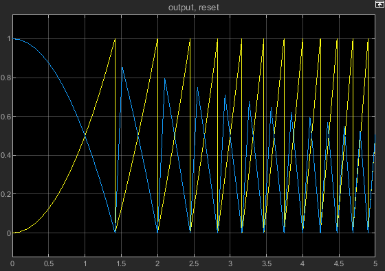
To view the output and reset signals in the Scope, double-click the Scope block. The Integrator block output signal oscillates between a value of 0 and 1. The output value resets to 0 each time the reset signal value is 0.
You can use the state port to prevent creating an algebraic loop when you need an Integrator block in one enabled subsystem to use the state of an Integrator block in another enabled subsystem.
Open the model EnabledSubsystemStatesAlgLoop.
mdl = "EnabledSubsystemStatesAlgLoop"; open_system(mdl)
The model contains two enabled subsystems, named A and B. A Pulse block provides the enable signal for both subsystems, but a Logical Operator block inverts the pulse to create the enable signal for subsystem A. As a result, the execution of the enabled subsystems alternates between subsystem A and subsystem B as the value of the Pulse block output changes.

Each enabled subsystem contains an Integrator block. To allow for continual integration of the input signal while execution alternates between the subsystems:
- The Enable block in each subsystem is configured to reset the subsystem states each time the subsystem executes.
- The Integrator block in each subsystem receives the initial state value through an input port that is connected to the output of the Integrator block in the other subsystem.

Connecting the output of one Integrator block to the input of the other creates an algebraic loop. To compute the output value from subsystem B, the solver needs the output from subsystem A and vice versa. To see the loop in the model, use the Simulink.BlockDiagram.getAlgebraicLoops function. The Algebraic Loops viewer opens and shows that the model contains one real algebraic loop.
Simulink.BlockDiagram.getAlgebraicLoops(mdl);

The algebraic loop is highlighted in the model.

If you try to simulate the model, the simulation issues an error during the initialization phase.
out = sim(mdl,CaptureErrors="on"); execinfo = out.SimulationMetadata.ExecutionInfo; stopreason = execinfo.StopEventDescription
stopreason = 'Error due to multiple causes.'
errphase = execinfo.ErrorDiagnostic.SimulationPhase
errphase = 'Initialization'
sldiagviewer.reportSimulationMetadataDiagnostics(out)
To pass states between the enabled subsystems without creating an algebraic loop, use the state port of the Integrator block. The solver computes the block state value at an earlier point in each time step, so the output for subsystem B no longer depends on the output from subsystem A and vice versa.
To see this solution, open the model EnabledSubsystemStates.
mdl2 = "EnabledSubsystemStates"; open_system(mdl2)
The input, enable, and output signals are the same, but the output from subsystem A no longer acts as a second input for subsystem B and vice versa.

To pass the states between the enabled subsystems:
- Each Integrator block is configured to show the state port.
- GoTo and From blocks with global visibility connect the state port of the Integrator block in subsystem A to the initial condition port of the Integrator block in subsystem B and vice versa.
The software does not support connecting the state port of an Integrator block to an output port of an enabled subsystem.

To verify that using the state port resolved the algebraic loop, use the Simulink.BlockDiagram.getAlgebraicLoops function.
Simulink.BlockDiagram.getAlgebraicLoops(mdl2);
No algebraic loops were found.
Simulate the model.
To view the results, double-click the Scope block. Alternatively, open the Scope window by calling the open_system function. The Scope window displays the enable signal and the output signals from each subsystem.
blk = mdl2 + "/Scope"; open_system(blk)

For another example of a system that passes Integrator state values between enabled subsystems, see Building a Clutch Lock-Up Model.
Extended Examples
Ports
Input
The input signal is a real-valued scalar, vector, or matrix that this block integrates.
This port does not have direct feedthrough.
Data Types: double
The external reset signal is a Boolean scalar, vector, or matrix that resets the block state to the initial condition. See Resetting the State.
This port has direct feedthrough.
Dependencies
To enable this port, select External Reset.
Data Types: Boolean
The initial condition signal is a real-valued scalar, vector, or matrix that sets the initial condition for the block.
This port has direct feedthrough.
Dependencies
To enable this port, set the Initial Conditions parameter toexternal.
Data Types: double
Output
The output signal is a scalar, vector, or matrix with the value of the integrated input signal. The dimensions of the integrated signal match the dimensions of the input signal.
Data Types: double
The output saturation signal is a scalar, vector, or matrix that indicates when each element in the block state is limited by the upper or lower saturation limit. The signal value indicates whether the value is limited and which limit is applied.
-1— Value limited by lower saturation limit0— Value not limited by either saturation limit1— Value limited by upper saturation limit
For more information, see Limiting the Integral.
Dependencies
To enable this port, select Show saturation port.
Data Types: double
The block state signal is a real-valued scalar, vector, or matrix with a value that matches the block state value.
For more information, see About the State Port.
Dependencies
To enable this port, select Show state port.
Data Types: double
Parameters
Specify the type of trigger to use for the external reset signal.
- Select
risingto reset the state when the reset signal rises from a negative or zero value to a positive value, or a negative value to zero value. - Select
fallingto reset the state when the reset signal falls from a positive value to a zero or negative value, or from a zero value to negative value. - Select
eitherto reset the state when the reset signal changes from zero to a nonzero value, from a nonzero value to zero, or changes sign. - Select
levelto reset the state when the reset signal is nonzero at the current time step or changes from nonzero at the previous time step to zero at the current time step. - Select
level holdto reset the state when the reset signal is nonzero at the current time step.
Programmatic Use
| **Block Parameter:**ExternalReset | ||||
|---|---|---|---|---|
| Type: character vector , string | ||||
| Values: 'none' | 'rising' | 'falling' | 'either' | 'level' | 'level hold' |
| Default: 'none' |
Select source of initial condition:
internal— Get the initial conditions of the states from the Initial condition parameter.external— Get the initial conditions of the states from an external signal. When you select this option, an input port appears on the block.
Programmatic Use
| **Block Parameter:**InitialConditionSource |
|---|
| Type: character vector, string |
| Values: 'internal' | 'external' |
| Default: 'internal' |
Set the initial state of the Integrator block.
Tips
Simulink software does not allow the initial condition of this block to beinf or NaN.
Dependencies
Setting Initial condition source tointernal enables this parameter.
Setting Initial condition source toexternal disables this parameter.
Programmatic Use
| **Block Parameter:**InitialCondition |
|---|
| Type: scalar or vector |
| Default: '0' |
Limit the block's output to a value between the Lower saturation limit and Upper saturation limit parameters.
- Selecting this check box limits the block output to a value between theLower saturation limit and Upper saturation limit parameters.
- Clearing this check box does not limit the block output values.
Dependencies
Selecting this parameter enables the Lower saturation limit and Upper saturation limit parameters.
Programmatic Use
| Block Parameter: LimitOutput |
|---|
| Type: character vector , string |
| Values: 'off' | 'on' |
| Default: 'off' |
Specify the upper limit for the integral as a scalar, vector, or matrix. You must specify a value between the Output minimum and Output maximum parameter values.
Dependencies
To enable this parameter, select theLimit output check box.
Programmatic Use
| Block Parameter: UpperSaturationLimit | |
|---|---|
| Type: character vector, string | |
| Values: scalar | vector | matrix |
| Default: 'inf' |
Specify the lower limit for the integral as a scalar, vector, or matrix. You must specify a value between the Output minimum and Output maximum parameter values.
Dependencies
To enable this parameter, select the Limit output check box.
Programmatic Use
| Block Parameter: LowerSaturationLimit | |
|---|---|
| Type: character vector , string | |
| Values: scalar | vector | matrix |
| Default: '-inf' |
Enable wrapping of states between the Wrapped state upper value and Wrapped state lower value parameters. Enabling wrap states eliminates the need for zero-crossing detection, reduces solver resets, improves solver performance and accuracy, and increases simulation time span when modeling rotary and cyclic state trajectories.
If you specify Wrapped state upper value asinf and Wrapped state lower value as-inf, wrapping does not occur.
Dependencies
Selecting this parameter enables Wrapped state upper value and Wrapped state lower value parameters.
Programmatic Use
| **Block Parameter:**WrapState |
|---|
| Type: character vector, string |
| Values: 'off' | 'on' |
| Default: 'off' |
Upper limit of the block output.
Dependencies
Selecting Wrap state enables this parameter.
Programmatic Use
| **Block Parameter:**WrappedStateUpperValue |
|---|
| Type: scalar or vector |
| Values: '2*pi' |
| Default: 'pi' |
Lower limit of the block output.
Dependencies
Selecting Wrap state enables this parameter.
Programmatic Use
| **Block Parameter:**WrappedStateLowerValue |
|---|
| Type: scalar or vector |
| Values: '0' |
| Default: '-pi' |
Select this check box to add a saturation output port to the block. When you clear this check box, the block does not have a saturation output port.
Dependencies
Selecting this parameter enables a saturation output port.
Programmatic Use
| Block Parameter: ShowSaturationPort |
|---|
| Type: character vector , string |
| Values: 'off' | 'on' |
| Default: 'off' |
Select this check box to add a state output port to the block. When you clear this check box, the block does not have a state output port.
Dependencies
Selecting this parameter enables a state output port.
Programmatic Use
| Block Parameter: ShowStatePort |
|---|
| Type: character vector , string |
| Values: 'off' | 'on' |
| Default: 'off' |
- If you enter
autoor –1, then Simulink uses the absolute tolerance value in the Configuration Parameters dialog box (see Solver Pane) to compute block states. - If you enter a real scalar, then that value overrides the absolute tolerance in the Configuration Parameters dialog box for computing all block states.
- If you enter a real vector, then the dimension of that vector must match the dimension of the continuous states in the block. These values override the absolute tolerance in the Configuration Parameters dialog box.
Programmatic Use
| Block Parameter: AbsoluteTolerance | |
|---|---|
| Type: character vector, string, scalar, or vector | |
| Values: 'auto' | '-1' | any positive real scalar or vector |
| Default: 'auto' |
When you select this parameter, the software ignores reset and limit parameters for this block during linearization and uses default values for those parameters.
Tip
Enable this parameter when you want to linearize a model around an operating point that causes the integrator to reset or saturate.
Programmatic Use
| Block Parameter: IgnoreLimit |
|---|
| Type: character vector | string |
| Values: 'off' | 'on' |
| Default: 'off' |
Select to enable zero-crossing detection. For more information, see Zero-Crossing Detection.
Programmatic Use
| Block Parameter:ZeroCross |
|---|
| Type: character vector | string |
| Values: 'off' |'on' |
| Default: 'on' |
- To assign a name to a single state, enter the name between quotes, for example,
'velocity'. - To assign names to multiple states, enter a comma-delimited list surrounded by braces, for example,
{'a', 'b', 'c'}. Each name must be unique. - The state names apply only to the selected block.
- The number of states must divide evenly among the number of state names.
- You can specify fewer names than states, but you cannot specify more names than states.
For example, you can specify two names in a system with four states. The first name applies to the first two states and the second name to the last two states. - To assign state names with a variable in the MATLAB® workspace, enter the variable without quotes. A variable can be a character vector, string, cell array, or structure.
Programmatic Use
| Block Parameter: ContinuousStateAttributes |
|---|
| Type: character vector, string |
| Values: ' ' | user-defined |
| Default: ' ' |
Block Characteristics
| Data Types | double |
|---|---|
| Direct Feedthrough | noa |
| Multidimensional Signals | no |
| Variable-Size Signals | no |
| Zero-Crossing Detection | yes |
| a Ports of this block have different direct feedthrough characteristics. |
Extended Capabilities
- Consider discretizing the model
- Not recommended for production code
Version History
Introduced before R2006a