plot - Plot Bayesian optimization results - MATLAB (original) (raw)
Plot Bayesian optimization results
Syntax
Description
plot([results](#bvbel%5Fv%5Fsep%5Fshared-results),'all') calls all predefined plot functions on results.
plot([results](#bvbel%5Fv%5Fsep%5Fshared-results),[plotFcn](#bvbel%5Fv-plotFcn)1,[plotFcn](#bvbel%5Fv-plotFcn)2,...) calls the listed plot functions on results.
Examples
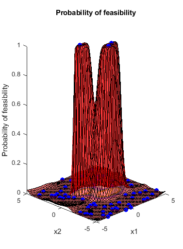
This example shows how to plot the error model and the best objective trace after the optimization has finished. The objective function for this example throws an error for points with norm larger than 2.
function f = makeanerror(x) f = x.x1 - x.x2 - sqrt(4-x.x1^2-x.x2^2);
Create the variables for optimization.
var1 = optimizableVariable('x1',[-5,5]); var2 = optimizableVariable('x2',[-5,5]); vars = [var1,var2];
Run the optimization without any plots. For reproducibility, set the random seed and use the 'expected-improvement-plus' acquisition function. Optimize for 60 iterations so the error model becomes well-trained.
rng default results = bayesopt(fun,vars,'MaxObjectiveEvaluations',60,... 'AcquisitionFunctionName','expected-improvement-plus',... 'PlotFcn',[],'Verbose',0);
Plot the error model and the best objective trace.
plot(results,@plotConstraintModels,@plotMinObjective)


Input Arguments
Plot function, specified as a function handle.
There are several built-in plot functions:
| Model Plots — Apply When D ≤ 2 | Description |
|---|---|
| @plotAcquisitionFunction | Plot the acquisition function surface. |
| @plotConstraintModels | Plot each constraint model surface. Negative values indicate feasible points.Also plot a_P_(feasible) surface.Also plot the error model, if it exists, which ranges from –1 to 1. Negative values mean that the model probably does not error, positive values mean that it probably does error. The model is:Plotted error = 2*Probability(error) – 1. |
| @plotObjectiveEvaluationTimeModel | Plot the objective function evaluation time model surface. |
| @plotObjectiveModel | Plot the fun model surface, the estimated location of the minimum, and the location of the next proposed point to evaluate. For one-dimensional problems, plot envelopes one credible interval above and below the mean function, and envelopes one noise standard deviation above and below the mean. |
| Trace Plots — Apply to All D | Description |
|---|---|
| @plotObjective | Plot each observed function value versus the number of function evaluations. |
| @plotObjectiveEvaluationTime | Plot each observed function evaluation run time versus the number of function evaluations. |
| @plotMinObjective | Plot the minimum observed and estimated function values versus the number of function evaluations. |
| @plotElapsedTime | Plot three curves: the total elapsed time of the optimization, the total function evaluation time, and the total modeling and point selection time, all versus the number of function evaluations. |
You can include a handle to your own plot functions. For details, seeBayesian Optimization Plot Functions.
Example: @plotObjective
Data Types: function_handle
Alternative Functionality
You can specify plot functions in the bayesopt PlotFcn name-value pair. This allows you to monitor the progress of the optimization.
Version History
Introduced in R2016b