numpy.meshgrid — NumPy v2.2 Manual (original) (raw)

numpy.meshgrid(*xi, copy=True, sparse=False, indexing='xy')[source]#

Return a tuple of coordinate matrices from coordinate vectors.

Make N-D coordinate arrays for vectorized evaluations of N-D scalar/vector fields over N-D grids, given one-dimensional coordinate arrays x1, x2,…, xn.

Parameters:

x1, x2,…, xnarray_like

1-D arrays representing the coordinates of a grid.

indexing{‘xy’, ‘ij’}, optional

Cartesian (‘xy’, default) or matrix (‘ij’) indexing of output. See Notes for more details.

sparsebool, optional

If True the shape of the returned coordinate array for dimension _i_is reduced from (N1, ..., Ni, ... Nn) to(1, ..., 1, Ni, 1, ..., 1). These sparse coordinate grids are intended to be use with Broadcasting. When all coordinates are used in an expression, broadcasting still leads to a fully-dimensonal result array.

Default is False.

copybool, optional

If False, a view into the original arrays are returned in order to conserve memory. Default is True. Please note thatsparse=False, copy=False will likely return non-contiguous arrays. Furthermore, more than one element of a broadcast array may refer to a single memory location. If you need to write to the arrays, make copies first.

Returns:

X1, X2,…, XNtuple of ndarrays

For vectors x1, x2,…, xn with lengths Ni=len(xi), returns (N1, N2, N3,..., Nn) shaped arrays if indexing=’ij’ or (N2, N1, N3,..., Nn) shaped arrays if indexing=’xy’ with the elements of xi repeated to fill the matrix along the first dimension for x1, the second for x2 and so on.

See also

mgrid

Construct a multi-dimensional “meshgrid” using indexing notation.

ogrid

Construct an open multi-dimensional “meshgrid” using indexing notation.

How to index ndarrays

Notes

This function supports both indexing conventions through the indexing keyword argument. Giving the string ‘ij’ returns a meshgrid with matrix indexing, while ‘xy’ returns a meshgrid with Cartesian indexing. In the 2-D case with inputs of length M and N, the outputs are of shape (N, M) for ‘xy’ indexing and (M, N) for ‘ij’ indexing. In the 3-D case with inputs of length M, N and P, outputs are of shape (N, M, P) for ‘xy’ indexing and (M, N, P) for ‘ij’ indexing. The difference is illustrated by the following code snippet:

xv, yv = np.meshgrid(x, y, indexing='ij') for i in range(nx): for j in range(ny): # treat xv[i,j], yv[i,j]

xv, yv = np.meshgrid(x, y, indexing='xy') for i in range(nx): for j in range(ny): # treat xv[j,i], yv[j,i]

In the 1-D and 0-D case, the indexing and sparse keywords have no effect.

Examples

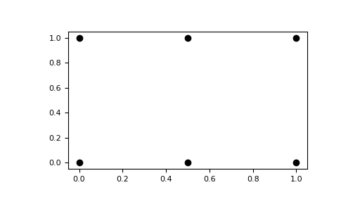
import numpy as np nx, ny = (3, 2) x = np.linspace(0, 1, nx) y = np.linspace(0, 1, ny) xv, yv = np.meshgrid(x, y) xv array([[0. , 0.5, 1. ], [0. , 0.5, 1. ]]) yv array([[0., 0., 0.], [1., 1., 1.]])

The result of meshgrid is a coordinate grid:

import matplotlib.pyplot as plt plt.plot(xv, yv, marker='o', color='k', linestyle='none') plt.show()

You can create sparse output arrays to save memory and computation time.

xv, yv = np.meshgrid(x, y, sparse=True) xv array([[0. , 0.5, 1. ]]) yv array([[0.], [1.]])

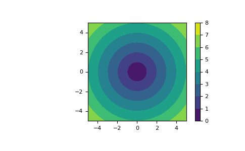
meshgrid is very useful to evaluate functions on a grid. If the function depends on all coordinates, both dense and sparse outputs can be used.

x = np.linspace(-5, 5, 101) y = np.linspace(-5, 5, 101)

full coordinate arrays

xx, yy = np.meshgrid(x, y) zz = np.sqrt(xx2 + yy2) xx.shape, yy.shape, zz.shape ((101, 101), (101, 101), (101, 101))

sparse coordinate arrays

xs, ys = np.meshgrid(x, y, sparse=True) zs = np.sqrt(xs2 + ys2) xs.shape, ys.shape, zs.shape ((1, 101), (101, 1), (101, 101)) np.array_equal(zz, zs) True

h = plt.contourf(x, y, zs) plt.axis('scaled') plt.colorbar() plt.show()