How to create arrays with regularly-spaced values — NumPy v2.2 Manual (original) (raw)

There are a few NumPy functions that are similar in application, but which provide slightly different results, which may cause confusion if one is not sure when and how to use them. The following guide aims to list these functions and describe their recommended usage.

The functions mentioned here are

• numpy.linspace
• numpy.arange
• numpy.geomspace
• numpy.logspace
• numpy.meshgrid
• numpy.mgrid
• numpy.ogrid

1D domains (intervals)#

linspace vs. arange#

Both numpy.linspace and numpy.arange provide ways to partition an interval (a 1D domain) into equal-length subintervals. These partitions will vary depending on the chosen starting and ending points, and the step (the length of the subintervals).

• Use numpy.arange if you want integer steps.
  numpy.arange relies on step size to determine how many elements are in the returned array, which excludes the endpoint. This is determined through thestep argument to arange.
  Example:

  np.arange(0, 10, 2) # np.arange(start, stop, step)
  array([0, 2, 4, 6, 8])
  The arguments start and stop should be integer or real, but not complex numbers. numpy.arange is similar to the Python built-inrange.
  Floating-point inaccuracies can make arange results with floating-point numbers confusing. In this case, you should use numpy.linspace instead.

• Use numpy.linspace if you want the endpoint to be included in the result, or if you are using a non-integer step size.
  numpy.linspace can include the endpoint and determines step size from the_num_ argument, which specifies the number of elements in the returned array.
  The inclusion of the endpoint is determined by an optional boolean argument endpoint, which defaults to True. Note that selectingendpoint=False will change the step size computation, and the subsequent output for the function.
  Example:

  np.linspace(0.1, 0.2, num=5) # np.linspace(start, stop, num)
  array([0.1 , 0.125, 0.15 , 0.175, 0.2 ])
  np.linspace(0.1, 0.2, num=5, endpoint=False)
  array([0.1, 0.12, 0.14, 0.16, 0.18])
  numpy.linspace can also be used with complex arguments:
  np.linspace(1+1.j, 4, 5, dtype=np.complex64)
  array([1. +1.j , 1.75+0.75j, 2.5 +0.5j , 3.25+0.25j, 4. +0.j ],
  dtype=complex64)

Other examples#

1. Unexpected results may happen if floating point values are used as stepin numpy.arange. To avoid this, make sure all floating point conversion happens after the computation of results. For example, replace

   list(np.arange(0.1,0.4,0.1).round(1))
   [0.1, 0.2, 0.3, 0.4] # endpoint should not be included!
   with
   list(np.arange(1, 4, 1) / 10.0)
   [0.1, 0.2, 0.3] # expected result

2. Note that

   np.arange(0, 1.12, 0.04)
   array([0. , 0.04, 0.08, 0.12, 0.16, 0.2 , 0.24, 0.28, 0.32, 0.36, 0.4 ,
   0.44, 0.48, 0.52, 0.56, 0.6 , 0.64, 0.68, 0.72, 0.76, 0.8 , 0.84,
   0.88, 0.92, 0.96, 1. , 1.04, 1.08, 1.12])

and

np.arange(0, 1.08, 0.04)
array([0. , 0.04, 0.08, 0.12, 0.16, 0.2 , 0.24, 0.28, 0.32, 0.36, 0.4 ,
0.44, 0.48, 0.52, 0.56, 0.6 , 0.64, 0.68, 0.72, 0.76, 0.8 , 0.84,
0.88, 0.92, 0.96, 1. , 1.04])
These differ because of numeric noise. When using floating point values, it is possible that 0 + 0.04 * 28 < 1.12, and so 1.12 is in the interval. In fact, this is exactly the case:
1.12/0.04
28.000000000000004
But 0 + 0.04 * 27 >= 1.08 so that 1.08 is excluded:
Alternatively, you could use np.arange(0, 28)*0.04 which would always give you precise control of the end point since it is integral:
np.arange(0, 28)*0.04
array([0. , 0.04, 0.08, 0.12, 0.16, 0.2 , 0.24, 0.28, 0.32, 0.36, 0.4 ,
0.44, 0.48, 0.52, 0.56, 0.6 , 0.64, 0.68, 0.72, 0.76, 0.8 , 0.84,
0.88, 0.92, 0.96, 1. , 1.04, 1.08])

geomspace and logspace#

numpy.geomspace is similar to numpy.linspace, but with numbers spaced evenly on a log scale (a geometric progression). The endpoint is included in the result.

Example:

np.geomspace(2, 3, num=5) array([2. , 2.21336384, 2.44948974, 2.71080601, 3. ])

numpy.logspace is similar to numpy.geomspace, but with the start and end points specified as logarithms (with base 10 as default):

np.logspace(2, 3, num=5) array([ 100. , 177.827941 , 316.22776602, 562.34132519, 1000. ])

In linear space, the sequence starts at base ** start (base to the power of start) and ends with base ** stop:

np.logspace(2, 3, num=5, base=2) array([4. , 4.75682846, 5.65685425, 6.72717132, 8. ])

N-D domains#

N-D domains can be partitioned into grids. This can be done using one of the following functions.

meshgrid#

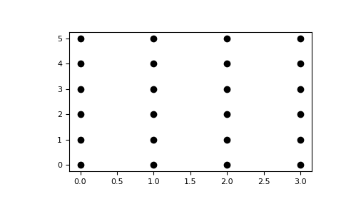
The purpose of numpy.meshgrid is to create a rectangular grid out of a set of one-dimensional coordinate arrays.

Given arrays:

x = np.array([0, 1, 2, 3]) y = np.array([0, 1, 2, 3, 4, 5])

meshgrid will create two coordinate arrays, which can be used to generate the coordinate pairs determining this grid.:

xx, yy = np.meshgrid(x, y) xx array([[0, 1, 2, 3], [0, 1, 2, 3], [0, 1, 2, 3], [0, 1, 2, 3], [0, 1, 2, 3], [0, 1, 2, 3]]) yy array([[0, 0, 0, 0], [1, 1, 1, 1], [2, 2, 2, 2], [3, 3, 3, 3], [4, 4, 4, 4], [5, 5, 5, 5]])

import matplotlib.pyplot as plt plt.plot(xx, yy, marker='.', color='k', linestyle='none')

mgrid#

numpy.mgrid can be used as a shortcut for creating meshgrids. It is not a function, but when indexed, returns a multidimensional meshgrid.

xx, yy = np.meshgrid(np.array([0, 1, 2, 3]), np.array([0, 1, 2, 3, 4, 5])) xx.T, yy.T (array([[0, 0, 0, 0, 0, 0], [1, 1, 1, 1, 1, 1], [2, 2, 2, 2, 2, 2], [3, 3, 3, 3, 3, 3]]), array([[0, 1, 2, 3, 4, 5], [0, 1, 2, 3, 4, 5], [0, 1, 2, 3, 4, 5], [0, 1, 2, 3, 4, 5]]))

np.mgrid[0:4, 0:6] array([[[0, 0, 0, 0, 0, 0], [1, 1, 1, 1, 1, 1], [2, 2, 2, 2, 2, 2], [3, 3, 3, 3, 3, 3]],

   [[0, 1, 2, 3, 4, 5],
    [0, 1, 2, 3, 4, 5],
    [0, 1, 2, 3, 4, 5],
    [0, 1, 2, 3, 4, 5]]])

ogrid#

Similar to numpy.mgrid, numpy.ogrid returns an open multidimensional meshgrid. This means that when it is indexed, only one dimension of each returned array is greater than 1. This avoids repeating the data and thus saves memory, which is often desirable.

These sparse coordinate grids are intended to be use with Broadcasting. When all coordinates are used in an expression, broadcasting still leads to a fully-dimensional result array.

np.ogrid[0:4, 0:6] (array([[0], [1], [2], [3]]), array([[0, 1, 2, 3, 4, 5]]))

All three methods described here can be used to evaluate function values on a grid.

g = np.ogrid[0:4, 0:6] zg = np.sqrt(g[0]**2 + g[1]**2) g[0].shape, g[1].shape, zg.shape ((4, 1), (1, 6), (4, 6)) m = np.mgrid[0:4, 0:6] zm = np.sqrt(m[0]**2 + m[1]**2) np.array_equal(zm, zg) True