arviz.kde — ArviZ dev documentation (original) (raw)

arviz.kde(x, circular=False, **kwargs)[source]#

One dimensional density estimation.

It is a wrapper around kde_linear() and kde_circular().

Parameters:

x1D numpy array

Data used to calculate the density estimation.

circularbool, optional

Whether x is a circular variable or not. Defaults to False.

kwargsdict, optional

Arguments passed to kde_linear() and kde_circular(). See their documentation for more info.

Returns:

gridnumpy.ndarray

Gridded numpy array for the x values.

pdfnumpy.ndarray

Numpy array for the density estimates.

bwfloat

The estimated bandwidth. Only returned if requested.

See also

plot_kde

Compute and plot a kernel density estimate.

Examples

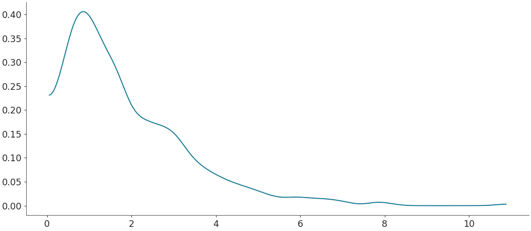
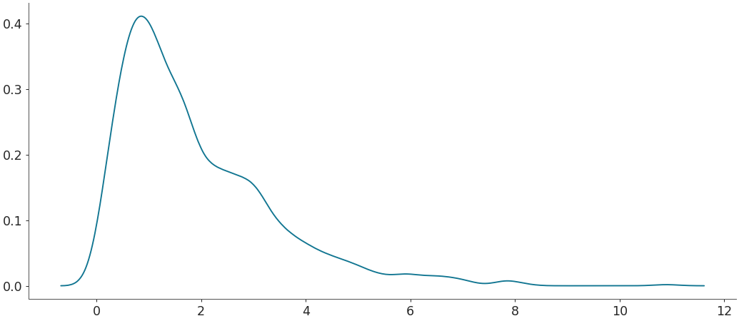
Default density estimation for linear data

import numpy as np import matplotlib.pyplot as plt from arviz import kde

rng = np.random.default_rng(49) rvs = rng.gamma(shape=1.8, size=1000) grid, pdf = kde(rvs) plt.plot(grid, pdf)

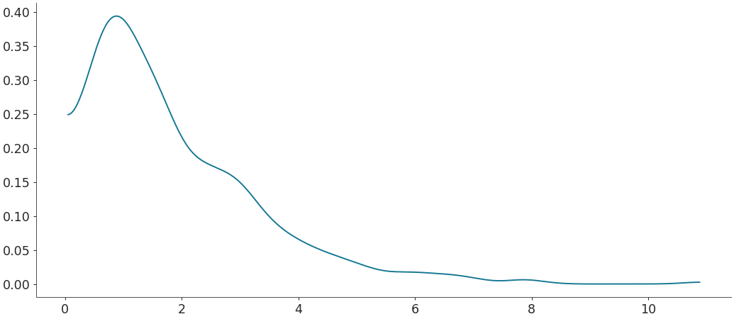
Density estimation for linear data with Silverman’s rule bandwidth

grid, pdf = kde(rvs, bw="silverman") plt.plot(grid, pdf)

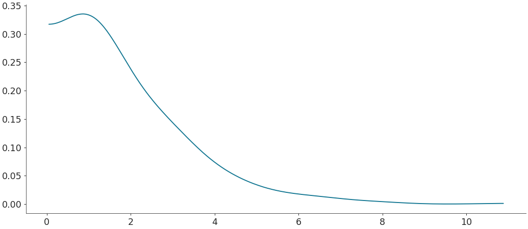
Density estimation for linear data with scaled bandwidth

bw_fct > 1 means more smoothness.

grid, pdf = kde(rvs, bw_fct=2.5) plt.plot(grid, pdf)

Default density estimation for linear data with extended limits

grid, pdf = kde(rvs, bound_correction=False, extend=True, extend_fct=0.5) plt.plot(grid, pdf)

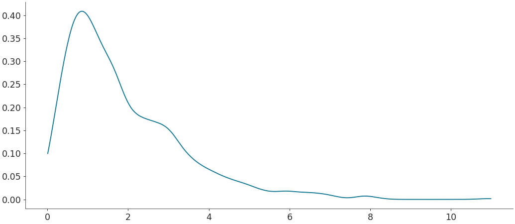
Default density estimation for linear data with custom limits

It accepts tuples and lists of length 2.

grid, pdf = kde(rvs, bound_correction=False, custom_lims=(0, 11)) plt.plot(grid, pdf)

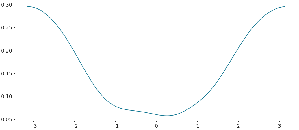
Default density estimation for circular data

rvs = np.random.vonmises(mu=np.pi, kappa=1, size=500) grid, pdf = kde(rvs, circular=True) plt.plot(grid, pdf)

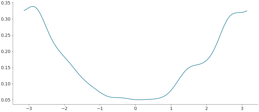
Density estimation for circular data with scaled bandwidth

rvs = np.random.vonmises(mu=np.pi, kappa=1, size=500)

bw_fct > 1 means less smoothness.

grid, pdf = kde(rvs, circular=True, bw_fct=3) plt.plot(grid, pdf)

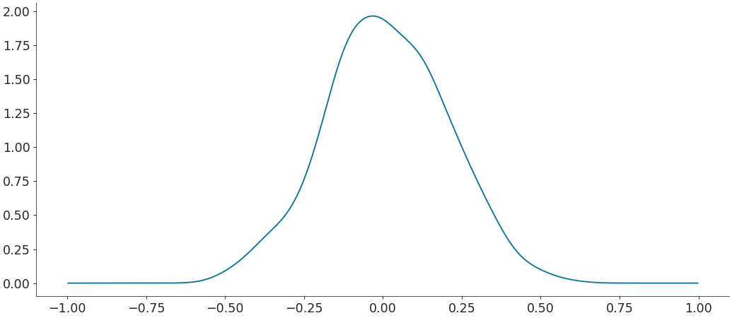
Density estimation for circular data with custom limits

This is still experimental, does not always work.

rvs = np.random.vonmises(mu=0, kappa=30, size=500) grid, pdf = kde(rvs, circular=True, custom_lims=(-1, 1)) plt.plot(grid, pdf)