arviz.plot_kde — ArviZ dev documentation (original) (raw)
arviz.plot_kde(values, values2=None, cumulative=False, rug=False, label=None, bw='default', adaptive=False, quantiles=None, rotated=False, contour=True, hdi_probs=None, fill_last=False, figsize=None, textsize=None, plot_kwargs=None, fill_kwargs=None, rug_kwargs=None, contour_kwargs=None, contourf_kwargs=None, pcolormesh_kwargs=None, is_circular=False, ax=None, legend=True, backend=None, backend_kwargs=None, show=None, return_glyph=False, **kwargs)[source]#
1D or 2D KDE plot taking into account boundary conditions.
Parameters:
valuesarray_like
Values to plot
values2array_like, optional
Values to plot. If present, a 2D KDE will be estimated
If True plot the estimated cumulative distribution function. Ignored for 2D KDE.
Add a rug plot for a specific subset of values. Ignored for 2D KDE.
labelstr, optional
Text to include as part of the legend.
If numeric, indicates the bandwidth and must be positive. If str, indicates the method to estimate the bandwidth and must be one of “scott”, “silverman”, “isj” or “experimental” when is_circular is False and “taylor” (for now) when is_circular is True. Defaults to “default” which means “experimental” when variable is not circular and “taylor” when it is.
If True, an adaptative bandwidth is used. Only valid for 1D KDE.
quantileslist, optional
Quantiles in ascending order used to segment the KDE. Use [.25, .5, .75] for quartiles.
Whether to rotate the 1D KDE plot 90 degrees.
If True plot the 2D KDE using contours, otherwise plot a smooth 2D KDE.
hdi_probslist, optional
Plots highest density credibility regions for the provided probabilities for a 2D KDE. Defaults to [0.5, 0.8, 0.94].
If True fill the last contour of the 2D KDE plot.
figsize(float, float), optional
Figure size. If None it will be defined automatically.
textsizefloat, optional
Text size scaling factor for labels, titles and lines. If None it will be autoscaled based on figsize. Not implemented for bokeh backend.
plot_kwargsdict, optional
Keywords passed to the pdf line of a 1D KDE. See matplotlib.axes.Axes.plot()or bokeh:bokeh.plotting.Figure.line() for a description of accepted values.
fill_kwargsdict, optional
Keywords passed to the fill under the line (use fill_kwargs={'alpha': 0}to disable fill). Ignored for 2D KDE. Passed tobokeh.plotting.Figure.patch().
rug_kwargsdict, optional
Keywords passed to the rug plot. Ignored if rug=False or for 2D KDE Use space keyword (float) to control the position of the rugplot. The larger this number the lower the rugplot. Passed to bokeh.models.glyphs.Scatter.
contour_kwargsdict, optional
Keywords passed to matplotlib.axes.Axes.contour()to draw contour lines or bokeh.plotting.Figure.patch(). Ignored for 1D KDE.
contourf_kwargsdict, optional
Keywords passed to matplotlib.axes.Axes.contourf()to draw filled contours. Ignored for 1D KDE.
pcolormesh_kwargsdict, optional
Keywords passed to matplotlib.axes.Axes.pcolormesh() orbokeh.plotting.Figure.image(). Ignored for 1D KDE.
is_circular{False, True, “radians”, “degrees”}. Default False
Select input type {“radians”, “degrees”} for circular histogram or KDE plot. If True, default input type is “radians”. When this argument is present, it interprets valuesas a circular variable measured in radians and a circular KDE is used. Inputs in “degrees” will undergo an internal conversion to radians.
axaxes, optional
Matplotlib axes or bokeh figures.
Add legend to the figure.
backend{“matplotlib”, “bokeh”}, default “matplotlib”
Select plotting backend.
backend_kwargsdict, optional
These are kwargs specific to the backend being used, passed tomatplotlib.pyplot.subplots() or bokeh.plotting.figure. For additional documentation check the plotting method of the backend.
showbool, optional
Call backend show function.
return_glyphbool, optional
Internal argument to return glyphs for bokeh.
Returns:
axesmatplotlib.Axes or bokeh.plotting.Figure
Object containing the kde plot
glyphslist, optional
Bokeh glyphs present in plot. Only provided if return_glyph is True.
See also
One dimensional density estimation.
Plot distribution as histogram or kernel density estimates.
Examples
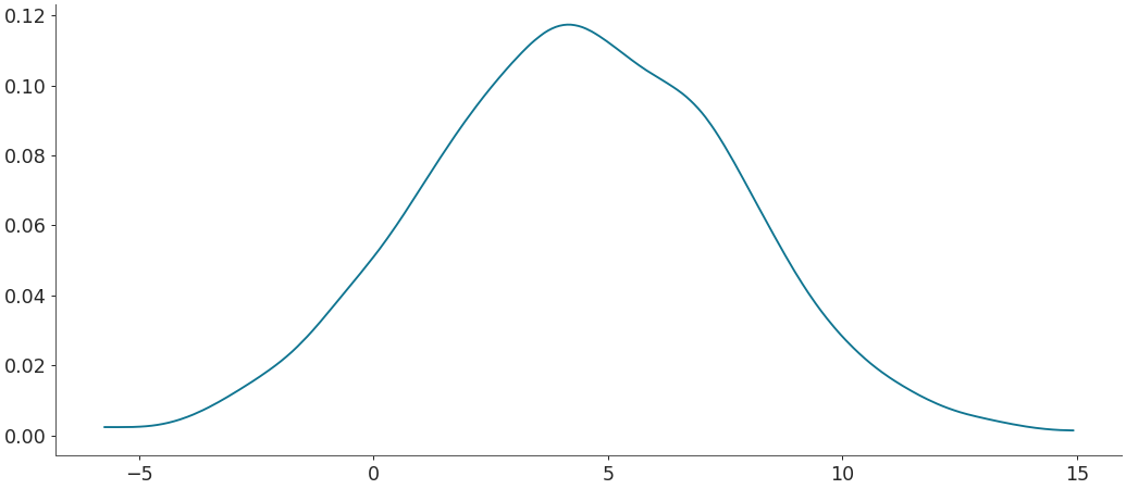
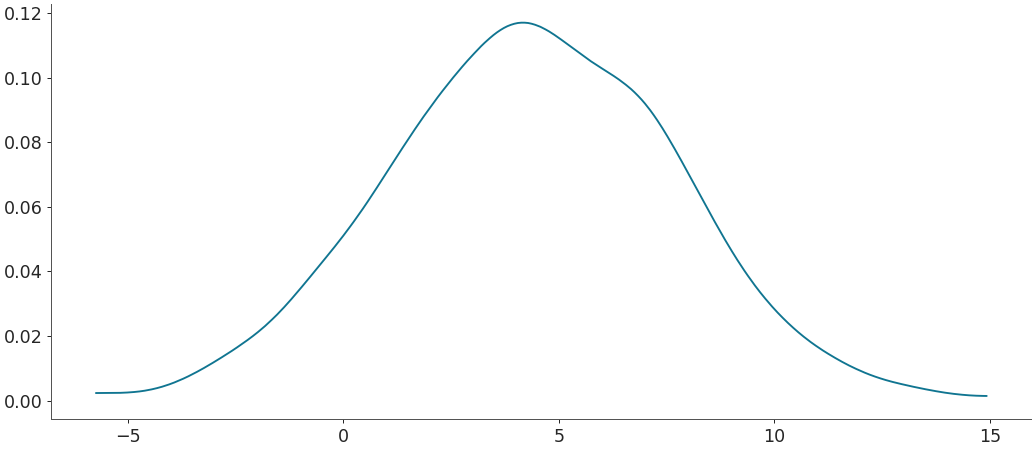
Plot default KDE
import arviz as az non_centered = az.load_arviz_data('non_centered_eight') mu_posterior = np.concatenate(non_centered.posterior["mu"].values) tau_posterior = np.concatenate(non_centered.posterior["tau"].values) az.plot_kde(mu_posterior)
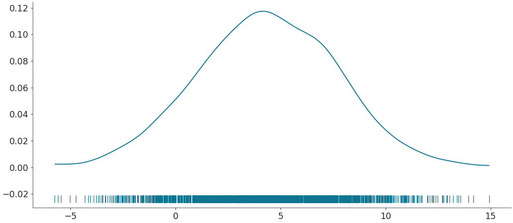
Plot KDE with rugplot
az.plot_kde(mu_posterior, rug=True)
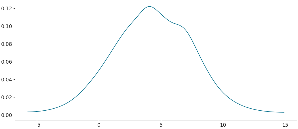
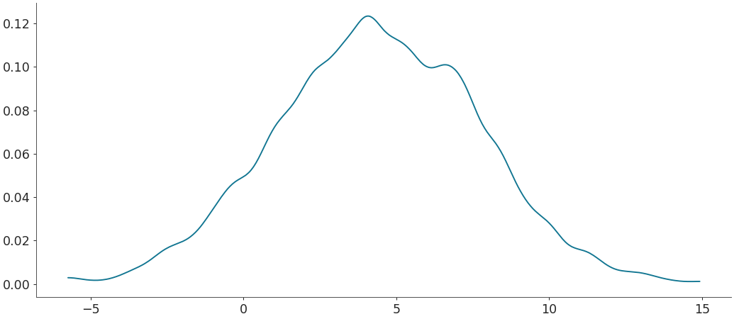
Plot KDE with adaptive bandwidth
az.plot_kde(mu_posterior, adaptive=True)
Plot KDE with a different bandwidth estimator
az.plot_kde(mu_posterior, bw="scott")
Plot KDE with a bandwidth specified manually
az.plot_kde(mu_posterior, bw=0.4)
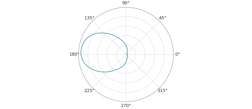
Plot KDE for a circular variable
rvs = np.random.vonmises(mu=np.pi, kappa=2, size=500) az.plot_kde(rvs, is_circular=True)
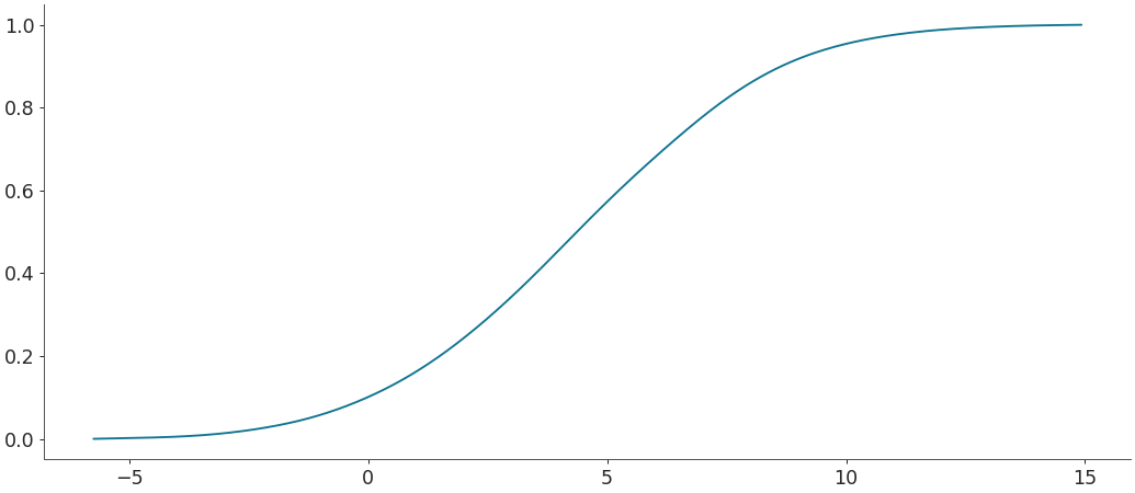
Plot a cumulative distribution
az.plot_kde(mu_posterior, cumulative=True)
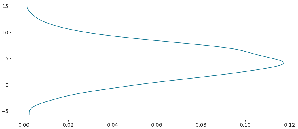
Rotate plot 90 degrees
az.plot_kde(mu_posterior, rotated=True)
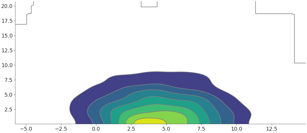
Plot 2d contour KDE
az.plot_kde(mu_posterior, values2=tau_posterior)
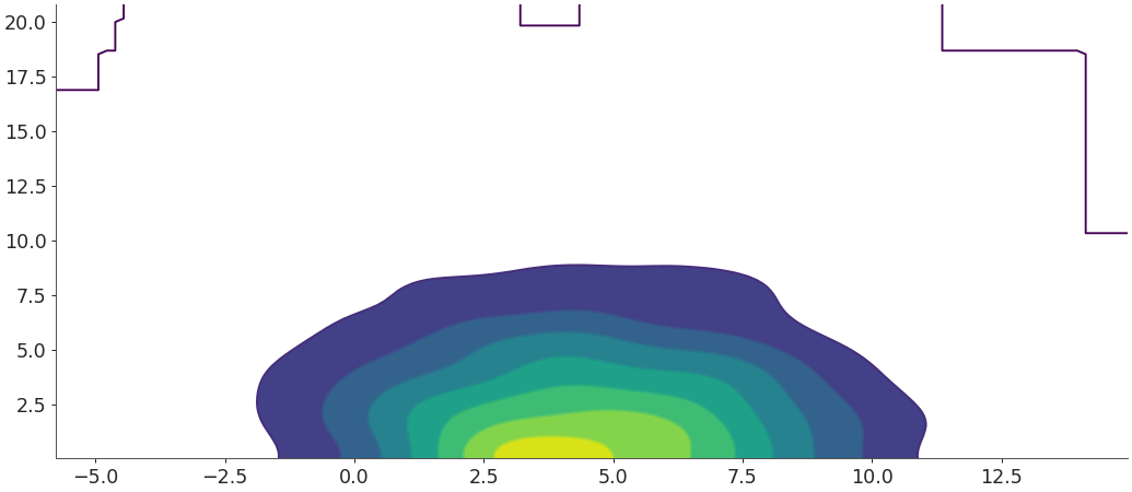
Plot 2d contour KDE, without filling and contour lines using viridis cmap
az.plot_kde(mu_posterior, values2=tau_posterior, ... contour_kwargs={"colors":None, "cmap":plt.cm.viridis}, ... contourf_kwargs={"alpha":0});
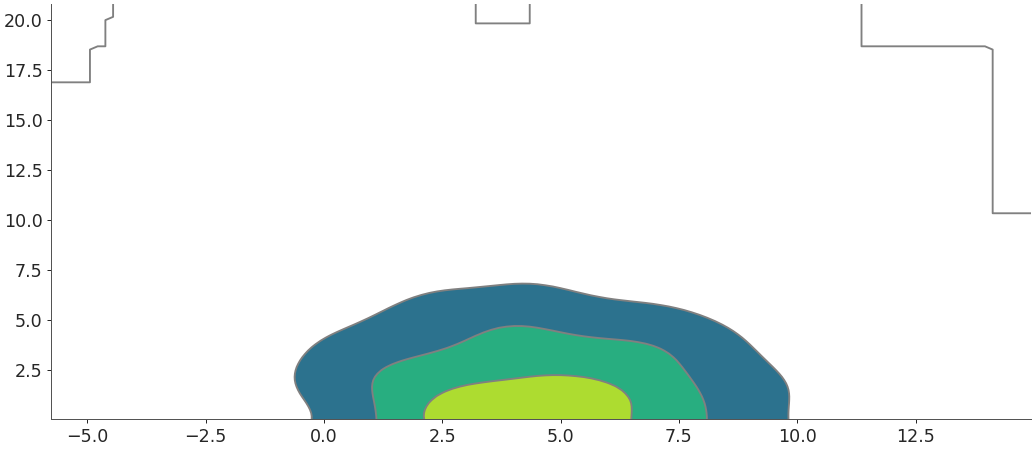
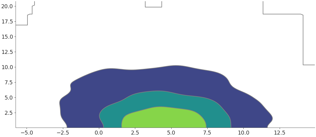
Plot 2d contour KDE, set the number of levels to 3.
az.plot_kde( ... mu_posterior, values2=tau_posterior, ... contour_kwargs={"levels":3}, contourf_kwargs={"levels":3} ... );
Plot 2d contour KDE with 30%, 60% and 90% HDI contours.
az.plot_kde(mu_posterior, values2=tau_posterior, hdi_probs=[0.3, 0.6, 0.9])
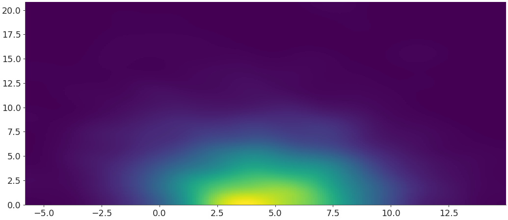
Plot 2d smooth KDE
az.plot_kde(mu_posterior, values2=tau_posterior, contour=False)