arviz.plot_bpv — ArviZ dev documentation (original) (raw)

arviz.plot_bpv(data, kind='u_value', t_stat='median', bpv=True, plot_mean=True, reference='analytical', smoothing=None, mse=False, n_ref=100, hdi_prob=0.94, color='C0', grid=None, figsize=None, textsize=None, labeller=None, data_pairs=None, var_names=None, filter_vars=None, coords=None, flatten=None, flatten_pp=None, ax=None, backend=None, plot_ref_kwargs=None, backend_kwargs=None, group='posterior', show=None)[source]#

Plot Bayesian p-value for observed data and Posterior/Prior predictive.

Parameters:

dataInferenceData

arviz.InferenceData object containing the observed and posterior/prior predictive data.

kind{“u_value”, “p_value”, “t_stat”}, default “u_value”

Specify the kind of plot:

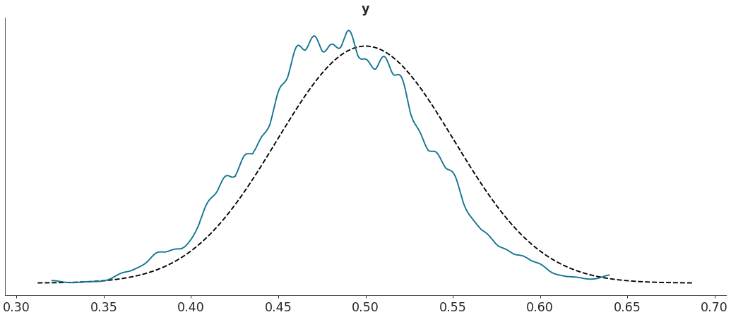
The kind="p_value" computes \(p := p(y* \leq y | y)\). This is the probability of the data y being larger or equal than the predicted data y*. The ideal value is 0.5 (half the predictions below and half above the data).
The kind="u_value" argument computes \(p_i := p(y_i* \leq y_i | y)\). i.e. like a p_value but per observation \(y_i\). This is also known as marginal p_value. The ideal distribution is uniform. This is similar to the LOO-PIT calculation/plot, the difference is than in LOO-pit plot we compute\(pi = p(y_i* r \leq y_i | y_{-i} )\), where \(y_{-i}\), is all other data except \(y_i\).
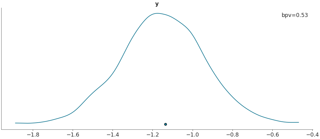
The kind="t_stat" argument computes \(:= p(T(y)* \leq T(y) | y)\)where T is any test statistic. See t_stat argument below for details of available options.

t_statstr, float, or callable(), default “median”

Test statistics to compute from the observations and predictive distributions. Allowed strings are “mean”, “median” or “std”. Alternative a quantile can be passed as a float (or str) in the interval (0, 1). Finally a user defined function is also acepted, see examples section for details.

bpvbool, default True

If True add the Bayesian p_value to the legend when kind = t_stat.

plot_meanbool, default True

Whether or not to plot the mean test statistic.

reference{“analytical”, “samples”, None}, default “analytical”

How to compute the distributions used as reference for kind=u_valuesor kind=p_values. Use None to not plot any reference.

smoothingbool, optional

If True and the data has integer dtype, smooth the data before computing the p-values, u-values or tstat. By default, True when kind is “u_value” and False otherwise.

msebool, default False

Show scaled mean square error between uniform distribution and marginal p_value distribution.

n_refint, default 100

Number of reference distributions to sample when reference=samples.

hdi_probfloat, optional

Probability for the highest density interval for the analytical reference distribution whenkind=u_values. Should be in the interval (0, 1]. Defaults to the rcParam stats.ci_prob. See this section for usage examples.

colorstr, optional

Matplotlib color

gridtuple, optional

Number of rows and columns. By default, the rows and columns are automatically inferred. See this section for usage examples.

figsize(float, float), optional

Figure size. If None it will be defined automatically.

textsizefloat, optional

Text size scaling factor for labels, titles and lines. If None it will be autoscaled based on figsize.

data_pairsdict, optional

Dictionary containing relations between observed data and posterior/prior predictive data. Dictionary structure:

key = data var_name
value = posterior/prior predictive var_name

For example, data_pairs = {'y' : 'y_hat'}If None, it will assume that the observed data and the posterior/prior predictive data have the same variable name.

LabellerLabeller, optional

Class providing the method make_pp_label to generate the labels in the plot titles. Read the Label guide for more details and usage examples.

var_nameslist of str, optional

Variables to be plotted. If None all variable are plotted. Prefix the variables by ~when you want to exclude them from the plot. See the this sectionfor usage examples. See this section for usage examples.

filter_vars{None, “like”, “regex”}, default None

If None (default), interpret var_names as the real variables names. If “like”, interpret var_names as substrings of the real variables names. If “regex”, interpret var_names as regular expressions on the real variables names. Seethis section for usage examples.

coordsdict, optional

Dictionary mapping dimensions to selected coordinates to be plotted. Dimensions without a mapping specified will include all coordinates for that dimension. Defaults to including all coordinates for all dimensions if None. See this section for usage examples.

flattenlist, optional

List of dimensions to flatten in observed_data. Only flattens across the coordinates specified in the coords argument. Defaults to flattening all of the dimensions.

flatten_pplist, optional

List of dimensions to flatten in posterior_predictive/prior_predictive. Only flattens across the coordinates specified in the coords argument. Defaults to flattening all of the dimensions. Dimensions should match flatten excluding dimensions for data_pairs parameters. If flatten is defined and flatten_pp is None, then flatten_pp=flatten.

legendbool, default True

Add legend to figure.

ax2D array_like of matplotlib Axes or Bokeh Figure, optional

A 2D array of locations into which to plot the densities. If not supplied, ArviZ will create its own array of plot areas (and return it).

backendstr, optional

Select plotting backend {“matplotlib”, “bokeh”}. Default “matplotlib”.

plot_ref_kwargsdict, optional

Extra keyword arguments to control how reference is represented. Passed to matplotlib.axes.Axes.plot() ormatplotlib.axes.Axes.axhspan() (when kind=u_valueand reference=analytical).

backend_kwargsbool, optional

These are kwargs specific to the backend being used, passed tomatplotlib.pyplot.subplots() or bokeh.plotting.figure. For additional documentation check the plotting method of the backend.

group{“posterior”, “prior”}, default “posterior”

Specifies which InferenceData group should be plotted. If “posterior”, then the values in posterior_predictive group are compared to the ones in observed_data, if “prior” then the same comparison happens, but with the values in prior_predictive group.

showbool, optional

Call backend show function.

Returns:

axes2D ndarray of matplotlib Axes or Bokeh Figure