arviz.plot_loo_pit — ArviZ dev documentation (original) (raw)
arviz.plot_loo_pit(idata=None, y=None, y_hat=None, log_weights=None, ecdf=False, ecdf_fill=True, n_unif=100, use_hdi=False, hdi_prob=None, figsize=None, textsize=None, labeller=None, color='C0', legend=True, ax=None, plot_kwargs=None, plot_unif_kwargs=None, hdi_kwargs=None, fill_kwargs=None, backend=None, backend_kwargs=None, show=None)[source]#
Plot Leave-One-Out (LOO) probability integral transformation (PIT) predictive checks.
Parameters:
idataInferenceData
arviz.InferenceData object.
Observed data. If str, idata must be present and contain the observed data group
Posterior predictive samples for y. It must have the same shape as y plus an extra dimension at the end of size n_samples (chains and draws stacked). If str or None, idata must contain the posterior predictive group. If None, y_hat is taken equal to y, thus, y must be str too.
Smoothed log_weights. It must have the same shape as y_hat
ecdfbool, optional
Plot the difference between the LOO-PIT Empirical Cumulative Distribution Function (ECDF) and the uniform CDF instead of LOO-PIT kde. In this case, instead of overlaying uniform distributions, the beta hdi_probaround the theoretical uniform CDF is shown. This approximation only holds for large S and ECDF values not very close to 0 nor 1. For more information, seeVehtari et al. (2021), Appendix G.
ecdf_fillbool, optional
Use matplotlib.axes.Axes.fill_between() to mark the area inside the credible interval. Otherwise, plot the border lines.
n_unifint, optional
Number of datasets to simulate and overlay from the uniform distribution.
use_hdibool, optional
Compute expected hdi values instead of overlaying the sampled uniform distributions.
hdi_probfloat, optional
Probability for the highest density interval. Works with use_hdi=True or ecdf=True.
figsize(float, float), optional
If None, size is (8 + numvars, 8 + numvars)
textsizeint, optional
Text size for labels. If None it will be autoscaled based on figsize.
labellerLabeller, optional
Class providing the method make_pp_label to generate the labels in the plot titles. Read the Label guide for more details and usage examples.
colorstr or array_like, optional
Color of the LOO-PIT estimated pdf plot. If plot_unif_kwargs has no “color” key, a slightly lighter color than this argument will be used for the uniform kde lines. This will ensure that LOO-PIT kde and uniform kde have different default colors.
legendbool, optional
Show the legend of the figure.
axaxes, optional
Matplotlib axes or bokeh figures.
plot_kwargsdict, optional
Additional keywords passed to matplotlib.axes.Axes.plot()for LOO-PIT line (kde or ECDF)
plot_unif_kwargsdict, optional
Additional keywords passed to matplotlib.axes.Axes.plot() for overlaid uniform distributions or for beta credible interval lines if ecdf=True
hdi_kwargsdict, optional
Additional keywords passed to matplotlib.axes.Axes.axhspan()
fill_kwargsdict, optional
Additional kwargs passed to matplotlib.axes.Axes.fill_between()
backendstr, optional
Select plotting backend {“matplotlib”,”bokeh”}. Default “matplotlib”.
backend_kwargsbool, optional
These are kwargs specific to the backend being used, passed tomatplotlib.pyplot.subplots() orbokeh.plotting.figure(). For additional documentation check the plotting method of the backend.
showbool, optional
Call backend show function.
Returns:
axesmatplotlib Axes or bokeh_figures
See also
Plot Bayesian p-value for observed data and Posterior/Prior predictive.
Compute leave one out (PSIS-LOO) probability integral transform (PIT) values.
References
- Gabry et al. (2017) see https://arxiv.org/abs/1709.01449
- https://mc-stan.org/bayesplot/reference/PPC-loo.html
- Gelman et al. BDA (2014) Section 6.3
Examples
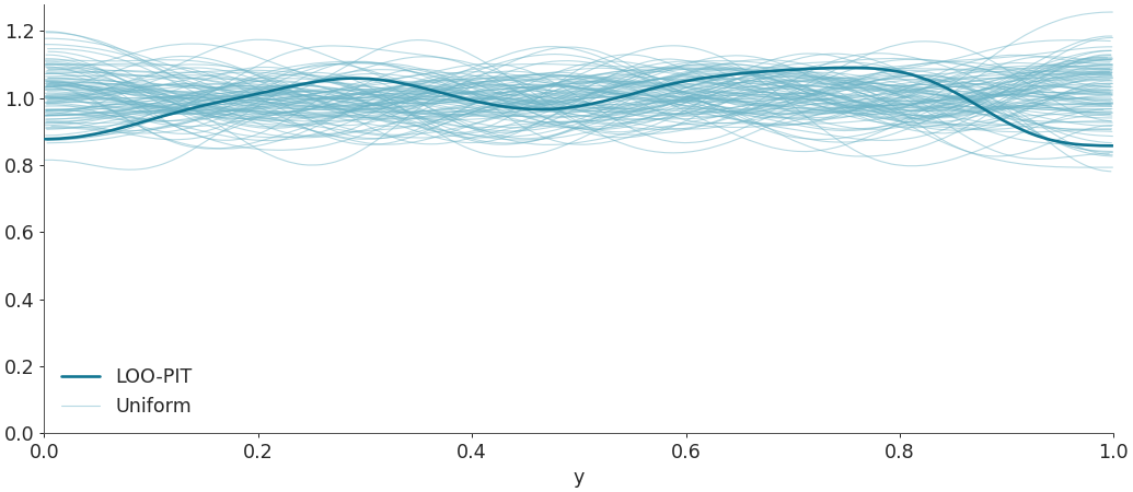
Plot LOO-PIT predictive checks overlaying the KDE of the LOO-PIT values to several realizations of uniform variable sampling with the same number of observations.
import arviz as az idata = az.load_arviz_data("radon") az.plot_loo_pit(idata=idata, y="y")
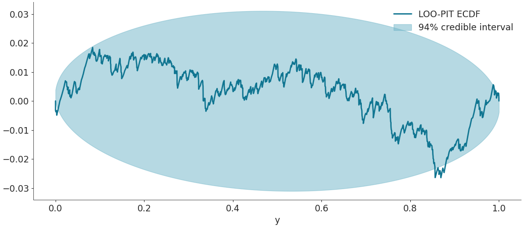
Fill the area containing the 94% highest density interval of the difference between uniform variables empirical CDF and the real uniform CDF. A LOO-PIT ECDF clearly outside of these theoretical boundaries indicates that the observations and the posterior predictive samples do not follow the same distribution.
az.plot_loo_pit(idata=idata, y="y", ecdf=True)