arviz.plot_ts — ArviZ dev documentation (original) (raw)
arviz.plot_ts(idata, y, x=None, y_hat=None, y_holdout=None, y_forecasts=None, x_holdout=None, plot_dim=None, holdout_dim=None, num_samples=100, backend=None, backend_kwargs=None, y_kwargs=None, y_hat_plot_kwargs=None, y_mean_plot_kwargs=None, vline_kwargs=None, textsize=None, figsize=None, legend=True, axes=None, show=None)[source]#
Plot timeseries data.
Parameters:
idataInferenceData
arviz.InferenceData object.
ystr
Variable name from observed_data. Values to be plotted on y-axis before holdout.
xstr, Optional
Values to be plotted on x-axis before holdout. If None, coords of y dims is chosen.
y_hatstr, optional
Variable name from posterior_predictive. Assumed to be of shape (chain, draw, *y_dims).
y_holdoutstr, optional
Variable name from observed_data. It represents the observed data after the holdout period. Useful while testing the model, when you want to compare observed test data with predictions/forecasts.
y_forecastsstr, optional
Variable name from posterior_predictive. It represents forecasts (posterior predictive) values after holdout period. Useful to compare observed vs predictions/forecasts. Assumed shape (chain, draw, *shape).
x_holdoutstr, Defaults to coords of y.
Variable name from constant_data. If None, coords of y_holdout or coords of y_forecast (either of the two available) is chosen.
plot_dim: str, Optional
Should be present in y.dims. Necessary for selection of x if x is None and y is multidimensional.
holdout_dim: str, Optional
Should be present in y_holdout.dims or y_forecats.dims. Necessary to choose x_holdout if x is None and if y_holdout or y_forecasts is multidimensional.
num_samplesint, default 100
Number of posterior predictive samples drawn from y_hat and y_forecasts.
backend{“matplotlib”, “bokeh”}, default “matplotlib”
Select plotting backend.
y_kwargsdict, optional
Passed to matplotlib.axes.Axes.plot() in matplotlib.
y_hat_plot_kwargsdict, optional
Passed to matplotlib.axes.Axes.plot() in matplotlib.
y_mean_plot_kwargsdict, optional
Passed to matplotlib.axes.Axes.plot() in matplotlib.
vline_kwargsdict, optional
Passed to matplotlib.axes.Axes.axvline() in matplotlib.
backend_kwargsdict, optional
These are kwargs specific to the backend being used. Passed tomatplotlib.pyplot.subplots().
figsizetuple, optional
Figure size. If None, it will be defined automatically.
textsizefloat, optional
Text size scaling factor for labels, titles and lines. If None, it will be autoscaled based on figsize.
Returns:
axes: matplotlib axes or bokeh figures.
See also
Posterior predictive and mean plots for regression-like data.
Plot for posterior/prior predictive checks.
Examples
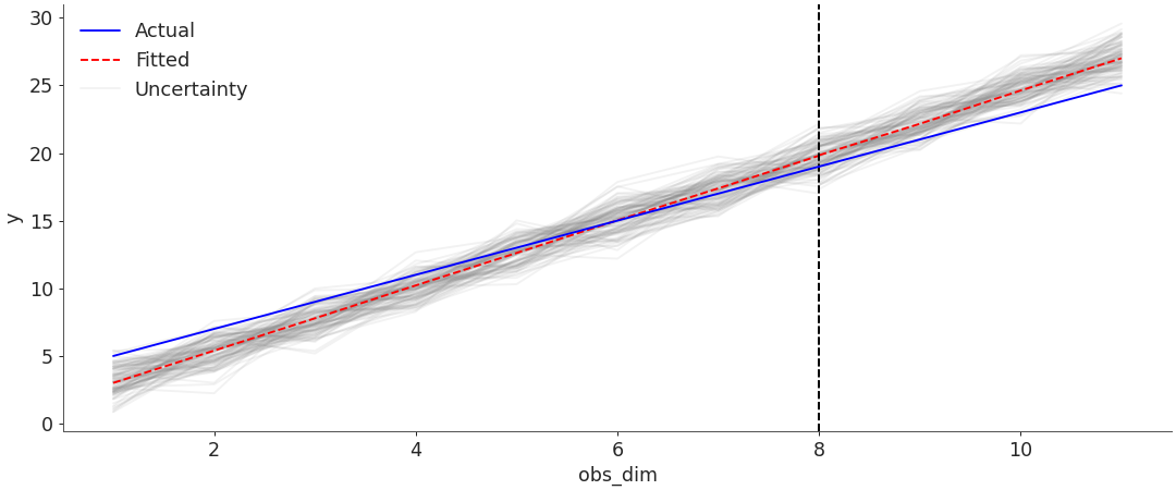
Plot timeseries default plot
import arviz as az nchains, ndraws = (4, 500) obs_data = { ... "y": 2 * np.arange(1, 9) + 3, ... "z": 2 * np.arange(8, 12) + 3, ... } posterior_predictive = { ... "y": np.random.normal( ... (obs_data["y"] * 1.2) - 3, size=(nchains, ndraws, len(obs_data["y"])) ... ), ... "z": np.random.normal( ... (obs_data["z"] * 1.2) - 3, size=(nchains, ndraws, len(obs_data["z"])) ... ), ... } idata = az.from_dict( ... observed_data=obs_data, ... posterior_predictive=posterior_predictive, ... coords={"obs_dim": np.arange(1, 9), "pred_dim": np.arange(8, 12)}, ... dims={"y": ["obs_dim"], "z": ["pred_dim"]}, ... ) ax = az.plot_ts(idata=idata, y="y", y_holdout="z")
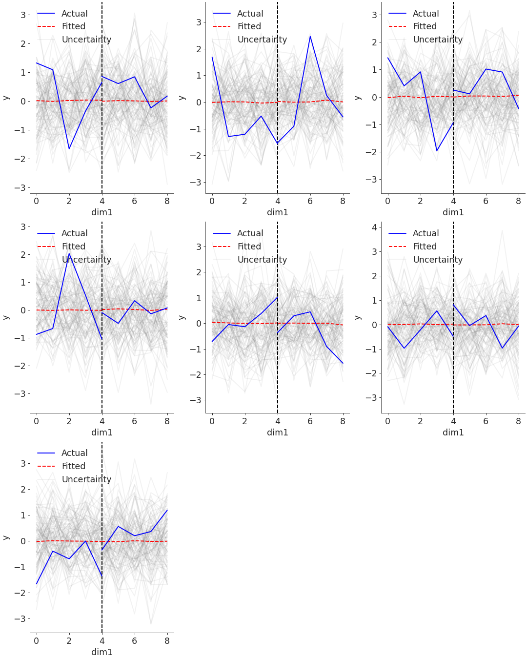
Plot timeseries multidim plot
ndim1, ndim2 = (5, 7) data = { ... "y": np.random.normal(size=(ndim1, ndim2)), ... "z": np.random.normal(size=(ndim1, ndim2)), ... } posterior_predictive = { ... "y": np.random.randn(nchains, ndraws, ndim1, ndim2), ... "z": np.random.randn(nchains, ndraws, ndim1, ndim2), ... } const_data = {"x": np.arange(1, 6), "x_pred": np.arange(5, 10)} idata = az.from_dict( ... observed_data=data, ... posterior_predictive=posterior_predictive, ... constant_data=const_data, ... dims={ ... "y": ["dim1", "dim2"], ... "z": ["holdout_dim1", "holdout_dim2"], ... }, ... coords={ ... "dim1": range(ndim1), ... "dim2": range(ndim2), ... "holdout_dim1": range(ndim1 - 1, ndim1 + 4), ... "holdout_dim2": range(ndim2 - 1, ndim2 + 6), ... }, ... ) az.plot_ts( ... idata=idata, ... y="y", ... plot_dim="dim1", ... y_holdout="z", ... holdout_dim="holdout_dim1", ... )