2.2. Manifold learning — scikit-learn 0.20.4 documentation (original) (raw)
Look for the bare necessities
The simple bare necessities
Forget about your worries and your strife
I mean the bare necessities
Old Mother Nature’s recipes
That bring the bare necessities of life
– Baloo’s song [The Jungle Book]
Manifold learning is an approach to non-linear dimensionality reduction. Algorithms for this task are based on the idea that the dimensionality of many data sets is only artificially high.
2.2.1. Introduction
High-dimensional datasets can be very difficult to visualize. While data in two or three dimensions can be plotted to show the inherent structure of the data, equivalent high-dimensional plots are much less intuitive. To aid visualization of the structure of a dataset, the dimension must be reduced in some way.
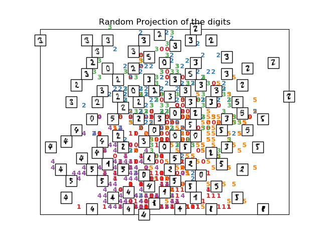
The simplest way to accomplish this dimensionality reduction is by taking a random projection of the data. Though this allows some degree of visualization of the data structure, the randomness of the choice leaves much to be desired. In a random projection, it is likely that the more interesting structure within the data will be lost.
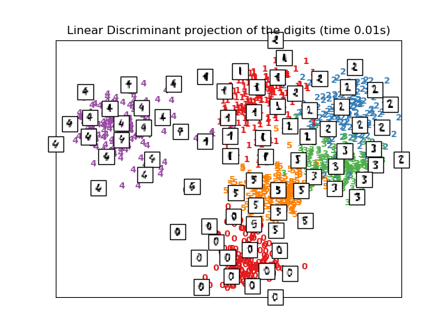
To address this concern, a number of supervised and unsupervised linear dimensionality reduction frameworks have been designed, such as Principal Component Analysis (PCA), Independent Component Analysis, Linear Discriminant Analysis, and others. These algorithms define specific rubrics to choose an “interesting” linear projection of the data. These methods can be powerful, but often miss important non-linear structure in the data.

Manifold Learning can be thought of as an attempt to generalize linear frameworks like PCA to be sensitive to non-linear structure in data. Though supervised variants exist, the typical manifold learning problem is unsupervised: it learns the high-dimensional structure of the data from the data itself, without the use of predetermined classifications.
Examples:
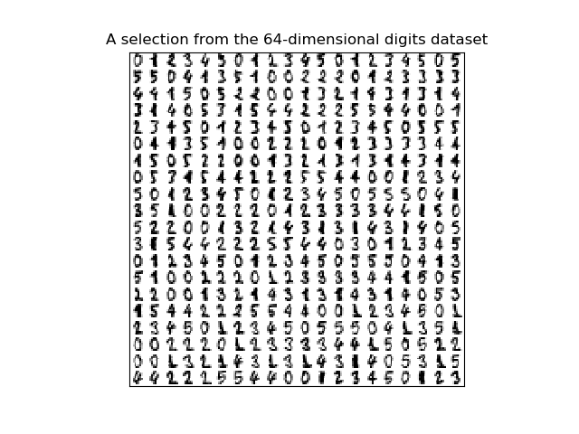
- See Manifold learning on handwritten digits: Locally Linear Embedding, Isomap… for an example of dimensionality reduction on handwritten digits.
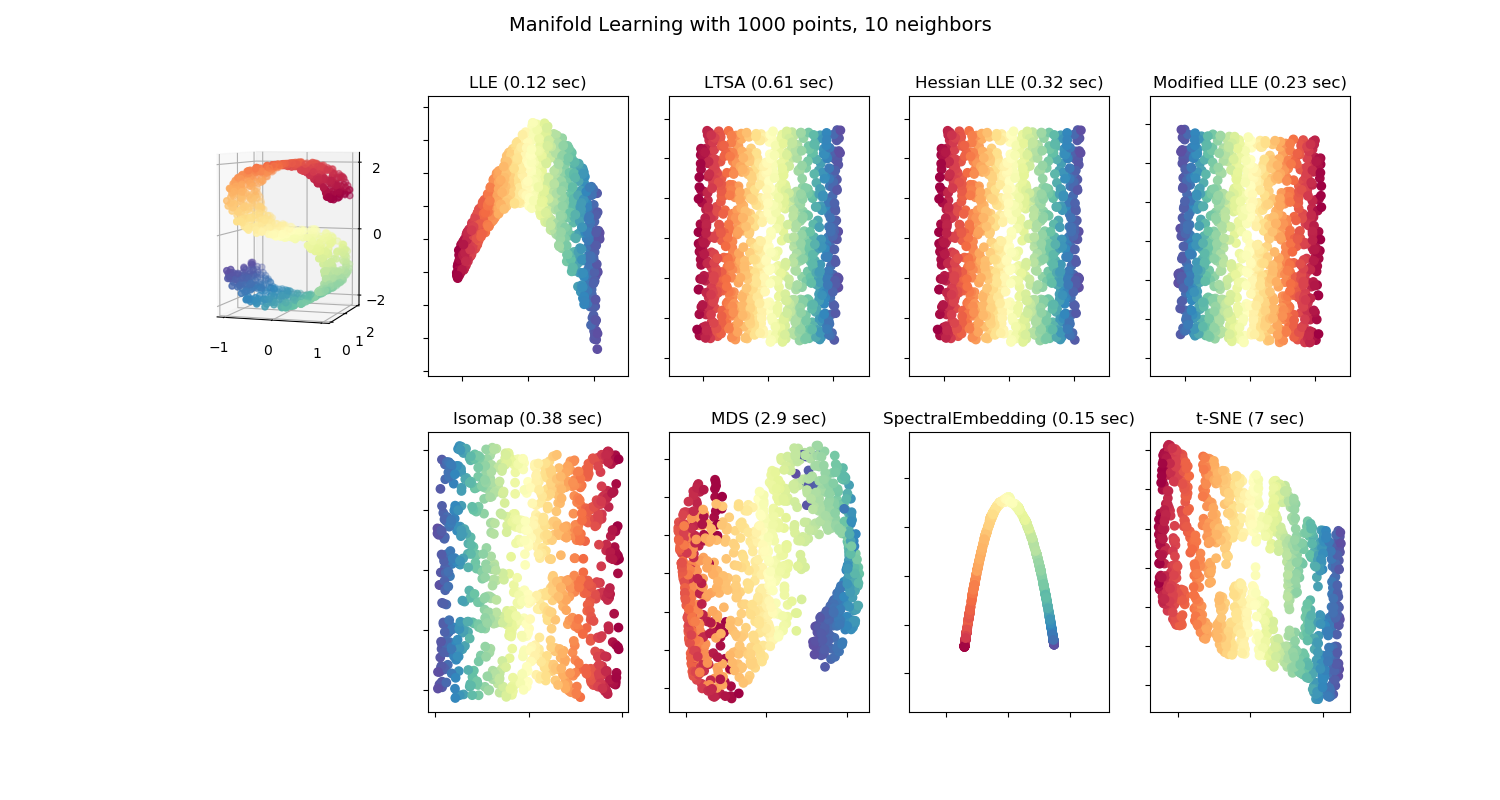
- See Comparison of Manifold Learning methods for an example of dimensionality reduction on a toy “S-curve” dataset.
The manifold learning implementations available in scikit-learn are summarized below
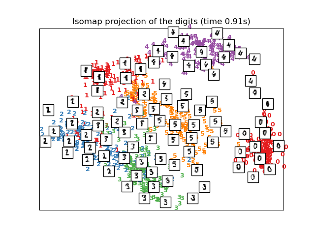
2.2.2. Isomap
One of the earliest approaches to manifold learning is the Isomap algorithm, short for Isometric Mapping. Isomap can be viewed as an extension of Multi-dimensional Scaling (MDS) or Kernel PCA. Isomap seeks a lower-dimensional embedding which maintains geodesic distances between all points. Isomap can be performed with the objectIsomap.
2.2.2.1. Complexity
The Isomap algorithm comprises three stages:
- Nearest neighbor search. Isomap usessklearn.neighbors.BallTree for efficient neighbor search. The cost is approximately \(O[D \log(k) N \log(N)]\), for \(k\)nearest neighbors of \(N\) points in \(D\) dimensions.
- Shortest-path graph search. The most efficient known algorithms for this are Dijkstra’s Algorithm, which is approximately\(O[N^2(k + \log(N))]\), or the Floyd-Warshall algorithm, which is \(O[N^3]\). The algorithm can be selected by the user with the
path_methodkeyword ofIsomap. If unspecified, the code attempts to choose the best algorithm for the input data. - Partial eigenvalue decomposition. The embedding is encoded in the eigenvectors corresponding to the \(d\) largest eigenvalues of the\(N \times N\) isomap kernel. For a dense solver, the cost is approximately \(O[d N^2]\). This cost can often be improved using the
ARPACKsolver. The eigensolver can be specified by the user with thepath_methodkeyword ofIsomap. If unspecified, the code attempts to choose the best algorithm for the input data.
The overall complexity of Isomap is\(O[D \log(k) N \log(N)] + O[N^2(k + \log(N))] + O[d N^2]\).
- \(N\) : number of training data points
- \(D\) : input dimension
- \(k\) : number of nearest neighbors
- \(d\) : output dimension
References:
- “A global geometric framework for nonlinear dimensionality reduction”Tenenbaum, J.B.; De Silva, V.; & Langford, J.C. Science 290 (5500)
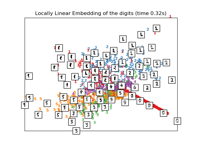
2.2.3. Locally Linear Embedding
Locally linear embedding (LLE) seeks a lower-dimensional projection of the data which preserves distances within local neighborhoods. It can be thought of as a series of local Principal Component Analyses which are globally compared to find the best non-linear embedding.
Locally linear embedding can be performed with functionlocally_linear_embedding or its object-oriented counterpartLocallyLinearEmbedding.
2.2.3.1. Complexity
The standard LLE algorithm comprises three stages:
- Nearest Neighbors Search. See discussion under Isomap above.
- Weight Matrix Construction. \(O[D N k^3]\). The construction of the LLE weight matrix involves the solution of a\(k \times k\) linear equation for each of the \(N\) local neighborhoods
- Partial Eigenvalue Decomposition. See discussion under Isomap above.
The overall complexity of standard LLE is\(O[D \log(k) N \log(N)] + O[D N k^3] + O[d N^2]\).
- \(N\) : number of training data points
- \(D\) : input dimension
- \(k\) : number of nearest neighbors
- \(d\) : output dimension
References:
- “Nonlinear dimensionality reduction by locally linear embedding”Roweis, S. & Saul, L. Science 290:2323 (2000)
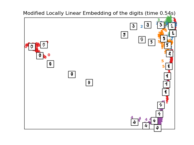
2.2.4. Modified Locally Linear Embedding
One well-known issue with LLE is the regularization problem. When the number of neighbors is greater than the number of input dimensions, the matrix defining each local neighborhood is rank-deficient. To address this, standard LLE applies an arbitrary regularization parameter \(r\), which is chosen relative to the trace of the local weight matrix. Though it can be shown formally that as \(r \to 0\), the solution converges to the desired embedding, there is no guarantee that the optimal solution will be found for \(r > 0\). This problem manifests itself in embeddings which distort the underlying geometry of the manifold.
One method to address the regularization problem is to use multiple weight vectors in each neighborhood. This is the essence of modified locally linear embedding (MLLE). MLLE can be performed with functionlocally_linear_embedding or its object-oriented counterpartLocallyLinearEmbedding, with the keyword method = 'modified'. It requires n_neighbors > n_components.
2.2.4.1. Complexity
The MLLE algorithm comprises three stages:
- Nearest Neighbors Search. Same as standard LLE
- Weight Matrix Construction. Approximately\(O[D N k^3] + O[N (k-D) k^2]\). The first term is exactly equivalent to that of standard LLE. The second term has to do with constructing the weight matrix from multiple weights. In practice, the added cost of constructing the MLLE weight matrix is relatively small compared to the cost of steps 1 and 3.
- Partial Eigenvalue Decomposition. Same as standard LLE
The overall complexity of MLLE is\(O[D \log(k) N \log(N)] + O[D N k^3] + O[N (k-D) k^2] + O[d N^2]\).
- \(N\) : number of training data points
- \(D\) : input dimension
- \(k\) : number of nearest neighbors
- \(d\) : output dimension
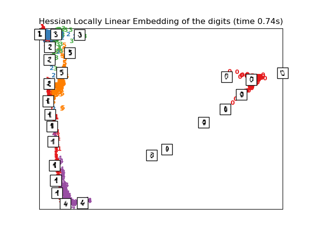
2.2.5. Hessian Eigenmapping
Hessian Eigenmapping (also known as Hessian-based LLE: HLLE) is another method of solving the regularization problem of LLE. It revolves around a hessian-based quadratic form at each neighborhood which is used to recover the locally linear structure. Though other implementations note its poor scaling with data size, sklearn implements some algorithmic improvements which make its cost comparable to that of other LLE variants for small output dimension. HLLE can be performed with functionlocally_linear_embedding or its object-oriented counterpartLocallyLinearEmbedding, with the keyword method = 'hessian'. It requires n_neighbors > n_components * (n_components + 3) / 2.
2.2.5.1. Complexity
The HLLE algorithm comprises three stages:
- Nearest Neighbors Search. Same as standard LLE
- Weight Matrix Construction. Approximately\(O[D N k^3] + O[N d^6]\). The first term reflects a similar cost to that of standard LLE. The second term comes from a QR decomposition of the local hessian estimator.
- Partial Eigenvalue Decomposition. Same as standard LLE
The overall complexity of standard HLLE is\(O[D \log(k) N \log(N)] + O[D N k^3] + O[N d^6] + O[d N^2]\).
- \(N\) : number of training data points
- \(D\) : input dimension
- \(k\) : number of nearest neighbors
- \(d\) : output dimension
References:
- “Hessian Eigenmaps: Locally linear embedding techniques for high-dimensional data”Donoho, D. & Grimes, C. Proc Natl Acad Sci USA. 100:5591 (2003)
2.2.6. Spectral Embedding
Spectral Embedding is an approach to calculating a non-linear embedding. Scikit-learn implements Laplacian Eigenmaps, which finds a low dimensional representation of the data using a spectral decomposition of the graph Laplacian. The graph generated can be considered as a discrete approximation of the low dimensional manifold in the high dimensional space. Minimization of a cost function based on the graph ensures that points close to each other on the manifold are mapped close to each other in the low dimensional space, preserving local distances. Spectral embedding can be performed with the function spectral_embedding or its object-oriented counterpartSpectralEmbedding.
2.2.6.1. Complexity
The Spectral Embedding (Laplacian Eigenmaps) algorithm comprises three stages:
- Weighted Graph Construction. Transform the raw input data into graph representation using affinity (adjacency) matrix representation.
- Graph Laplacian Construction. unnormalized Graph Laplacian is constructed as \(L = D - A\) for and normalized one as\(L = D^{-\frac{1}{2}} (D - A) D^{-\frac{1}{2}}\).
- Partial Eigenvalue Decomposition. Eigenvalue decomposition is done on graph Laplacian
The overall complexity of spectral embedding is\(O[D \log(k) N \log(N)] + O[D N k^3] + O[d N^2]\).
- \(N\) : number of training data points
- \(D\) : input dimension
- \(k\) : number of nearest neighbors
- \(d\) : output dimension
References:
- “Laplacian Eigenmaps for Dimensionality Reduction and Data Representation”M. Belkin, P. Niyogi, Neural Computation, June 2003; 15 (6):1373-1396
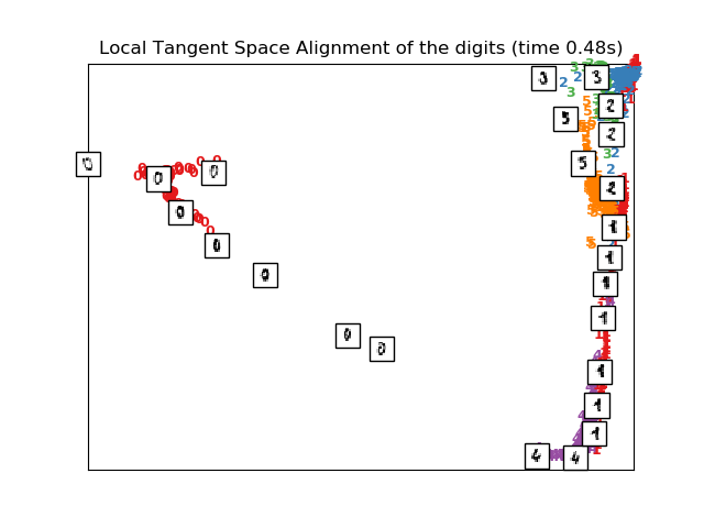
2.2.7. Local Tangent Space Alignment
Though not technically a variant of LLE, Local tangent space alignment (LTSA) is algorithmically similar enough to LLE that it can be put in this category. Rather than focusing on preserving neighborhood distances as in LLE, LTSA seeks to characterize the local geometry at each neighborhood via its tangent space, and performs a global optimization to align these local tangent spaces to learn the embedding. LTSA can be performed with functionlocally_linear_embedding or its object-oriented counterpartLocallyLinearEmbedding, with the keyword method = 'ltsa'.
2.2.7.1. Complexity
The LTSA algorithm comprises three stages:
- Nearest Neighbors Search. Same as standard LLE
- Weight Matrix Construction. Approximately\(O[D N k^3] + O[k^2 d]\). The first term reflects a similar cost to that of standard LLE.
- Partial Eigenvalue Decomposition. Same as standard LLE
The overall complexity of standard LTSA is\(O[D \log(k) N \log(N)] + O[D N k^3] + O[k^2 d] + O[d N^2]\).
- \(N\) : number of training data points
- \(D\) : input dimension
- \(k\) : number of nearest neighbors
- \(d\) : output dimension
References:
- “Principal manifolds and nonlinear dimensionality reduction via tangent space alignment”Zhang, Z. & Zha, H. Journal of Shanghai Univ. 8:406 (2004)
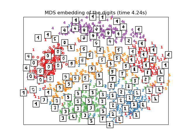
2.2.8. Multi-dimensional Scaling (MDS)
Multidimensional scaling(MDS) seeks a low-dimensional representation of the data in which the distances respect well the distances in the original high-dimensional space.
In general, is a technique used for analyzing similarity or dissimilarity data. MDS attempts to model similarity or dissimilarity data as distances in a geometric spaces. The data can be ratings of similarity between objects, interaction frequencies of molecules, or trade indices between countries.
There exists two types of MDS algorithm: metric and non metric. In the scikit-learn, the class MDS implements both. In Metric MDS, the input similarity matrix arises from a metric (and thus respects the triangular inequality), the distances between output two points are then set to be as close as possible to the similarity or dissimilarity data. In the non-metric version, the algorithms will try to preserve the order of the distances, and hence seek for a monotonic relationship between the distances in the embedded space and the similarities/dissimilarities.
Let \(S\) be the similarity matrix, and \(X\) the coordinates of the\(n\) input points. Disparities \(\hat{d}_{ij}\) are transformation of the similarities chosen in some optimal ways. The objective, called the stress, is then defined by \(sum_{i < j} d_{ij}(X) - \hat{d}_{ij}(X)\)
2.2.8.1. Metric MDS
The simplest metric MDS model, called absolute MDS, disparities are defined by\(\hat{d}_{ij} = S_{ij}\). With absolute MDS, the value \(S_{ij}\)should then correspond exactly to the distance between point \(i\) and\(j\) in the embedding point.
Most commonly, disparities are set to \(\hat{d}_{ij} = b S_{ij}\).
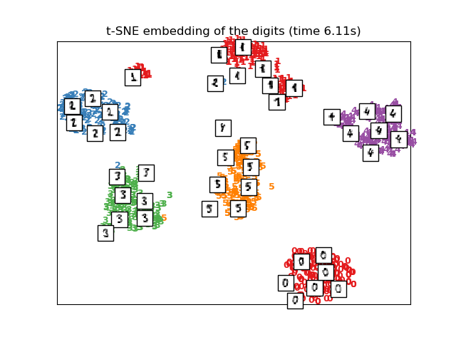
2.2.9. t-distributed Stochastic Neighbor Embedding (t-SNE)
t-SNE (TSNE) converts affinities of data points to probabilities. The affinities in the original space are represented by Gaussian joint probabilities and the affinities in the embedded space are represented by Student’s t-distributions. This allows t-SNE to be particularly sensitive to local structure and has a few other advantages over existing techniques:
- Revealing the structure at many scales on a single map
- Revealing data that lie in multiple, different, manifolds or clusters
- Reducing the tendency to crowd points together at the center
While Isomap, LLE and variants are best suited to unfold a single continuous low dimensional manifold, t-SNE will focus on the local structure of the data and will tend to extract clustered local groups of samples as highlighted on the S-curve example. This ability to group samples based on the local structure might be beneficial to visually disentangle a dataset that comprises several manifolds at once as is the case in the digits dataset.
The Kullback-Leibler (KL) divergence of the joint probabilities in the original space and the embedded space will be minimized by gradient descent. Note that the KL divergence is not convex, i.e. multiple restarts with different initializations will end up in local minima of the KL divergence. Hence, it is sometimes useful to try different seeds and select the embedding with the lowest KL divergence.
The disadvantages to using t-SNE are roughly:
- t-SNE is computationally expensive, and can take several hours on million-sample datasets where PCA will finish in seconds or minutes
- The Barnes-Hut t-SNE method is limited to two or three dimensional embeddings.
- The algorithm is stochastic and multiple restarts with different seeds can yield different embeddings. However, it is perfectly legitimate to pick the embedding with the least error.
- Global structure is not explicitly preserved. This is problem is mitigated by initializing points with PCA (using init=’pca’).
2.2.9.1. Optimizing t-SNE
The main purpose of t-SNE is visualization of high-dimensional data. Hence, it works best when the data will be embedded on two or three dimensions.
Optimizing the KL divergence can be a little bit tricky sometimes. There are five parameters that control the optimization of t-SNE and therefore possibly the quality of the resulting embedding:
- perplexity
- early exaggeration factor
- learning rate
- maximum number of iterations
- angle (not used in the exact method)
The perplexity is defined as \(k=2^{(S)}\) where \(S\) is the Shannon entropy of the conditional probability distribution. The perplexity of a\(k\)-sided die is \(k\), so that \(k\) is effectively the number of nearest neighbors t-SNE considers when generating the conditional probabilities. Larger perplexities lead to more nearest neighbors and less sensitive to small structure. Conversely a lower perplexity considers a smaller number of neighbors, and thus ignores more global information in favour of the local neighborhood. As dataset sizes get larger more points will be required to get a reasonable sample of the local neighborhood, and hence larger perplexities may be required. Similarly noisier datasets will require larger perplexity values to encompass enough local neighbors to see beyond the background noise.
The maximum number of iterations is usually high enough and does not need any tuning. The optimization consists of two phases: the early exaggeration phase and the final optimization. During early exaggeration the joint probabilities in the original space will be artificially increased by multiplication with a given factor. Larger factors result in larger gaps between natural clusters in the data. If the factor is too high, the KL divergence could increase during this phase. Usually it does not have to be tuned. A critical parameter is the learning rate. If it is too low gradient descent will get stuck in a bad local minimum. If it is too high the KL divergence will increase during optimization. More tips can be found in Laurens van der Maaten’s FAQ (see references). The last parameter, angle, is a tradeoff between performance and accuracy. Larger angles imply that we can approximate larger regions by a single point, leading to better speed but less accurate results.
“How to Use t-SNE Effectively”provides a good discussion of the effects of the various parameters, as well as interactive plots to explore the effects of different parameters.
2.2.9.2. Barnes-Hut t-SNE
The Barnes-Hut t-SNE that has been implemented here is usually much slower than other manifold learning algorithms. The optimization is quite difficult and the computation of the gradient is \(O[d N log(N)]\), where \(d\)is the number of output dimensions and \(N\) is the number of samples. The Barnes-Hut method improves on the exact method where t-SNE complexity is\(O[d N^2]\), but has several other notable differences:
- The Barnes-Hut implementation only works when the target dimensionality is 3 or less. The 2D case is typical when building visualizations.
- Barnes-Hut only works with dense input data. Sparse data matrices can only be embedded with the exact method or can be approximated by a dense low rank projection for instance using sklearn.decomposition.TruncatedSVD
- Barnes-Hut is an approximation of the exact method. The approximation is parameterized with the angle parameter, therefore the angle parameter is unused when method=”exact”
- Barnes-Hut is significantly more scalable. Barnes-Hut can be used to embed hundred of thousands of data points while the exact method can handle thousands of samples before becoming computationally intractable
For visualization purpose (which is the main use case of t-SNE), using the Barnes-Hut method is strongly recommended. The exact t-SNE method is useful for checking the theoretically properties of the embedding possibly in higher dimensional space but limit to small datasets due to computational constraints.
Also note that the digits labels roughly match the natural grouping found by t-SNE while the linear 2D projection of the PCA model yields a representation where label regions largely overlap. This is a strong clue that this data can be well separated by non linear methods that focus on the local structure (e.g. an SVM with a Gaussian RBF kernel). However, failing to visualize well separated homogeneously labeled groups with t-SNE in 2D does not necessarily imply that the data cannot be correctly classified by a supervised model. It might be the case that 2 dimensions are not low enough to accurately represents the internal structure of the data.
References:
- “Visualizing High-Dimensional Data Using t-SNE”van der Maaten, L.J.P.; Hinton, G. Journal of Machine Learning Research (2008)
- “t-Distributed Stochastic Neighbor Embedding”van der Maaten, L.J.P.
- “Accelerating t-SNE using Tree-Based Algorithms.”L.J.P. van der Maaten. Journal of Machine Learning Research 15(Oct):3221-3245, 2014.
2.2.10. Tips on practical use
- Make sure the same scale is used over all features. Because manifold learning methods are based on a nearest-neighbor search, the algorithm may perform poorly otherwise. See StandardScalerfor convenient ways of scaling heterogeneous data.
- The reconstruction error computed by each routine can be used to choose the optimal output dimension. For a \(d\)-dimensional manifold embedded in a \(D\)-dimensional parameter space, the reconstruction error will decrease as
n_componentsis increased untiln_components == d. - Note that noisy data can “short-circuit” the manifold, in essence acting as a bridge between parts of the manifold that would otherwise be well-separated. Manifold learning on noisy and/or incomplete data is an active area of research.
- Certain input configurations can lead to singular weight matrices, for example when more than two points in the dataset are identical, or when the data is split into disjointed groups. In this case,
solver='arpack'will fail to find the null space. The easiest way to address this is to usesolver='dense'which will work on a singular matrix, though it may be very slow depending on the number of input points. Alternatively, one can attempt to understand the source of the singularity: if it is due to disjoint sets, increasingn_neighborsmay help. If it is due to identical points in the dataset, removing these points may help.
See also
Totally Random Trees Embedding can also be useful to derive non-linear representations of feature space, also it does not perform dimensionality reduction.