Introducing the set_output API (original) (raw)
Note
Go to the endto download the full example code or to run this example in your browser via JupyterLite or Binder.
This example will demonstrate the set_output API to configure transformers to output pandas DataFrames. set_output can be configured per estimator by calling the set_output method or globally by setting set_config(transform_output="pandas"). For details, seeSLEP018.
First, we load the iris dataset as a DataFrame to demonstrate the set_output API.
| sepal length (cm) | sepal width (cm) | petal length (cm) | petal width (cm) | |
|---|---|---|---|---|
| 60 | 5.0 | 2.0 | 3.5 | 1.0 |
| 1 | 4.9 | 3.0 | 1.4 | 0.2 |
| 8 | 4.4 | 2.9 | 1.4 | 0.2 |
| 93 | 5.0 | 2.3 | 3.3 | 1.0 |
| 106 | 4.9 | 2.5 | 4.5 | 1.7 |
To configure an estimator such as preprocessing.StandardScaler to return DataFrames, call set_output. This feature requires pandas to be installed.
from sklearn.preprocessing import StandardScaler
scaler = StandardScaler().set_output(transform="pandas")
scaler.fit(X_train) X_test_scaled = scaler.transform(X_test) X_test_scaled.head()
| sepal length (cm) | sepal width (cm) | petal length (cm) | petal width (cm) | |
|---|---|---|---|---|
| 39 | -0.894264 | 0.798301 | -1.271411 | -1.327605 |
| 12 | -1.244466 | -0.086944 | -1.327407 | -1.459074 |
| 48 | -0.660797 | 1.462234 | -1.271411 | -1.327605 |
| 23 | -0.894264 | 0.576989 | -1.159419 | -0.933197 |
| 81 | -0.427329 | -1.414810 | -0.039497 | -0.275851 |
set_output can be called after fit to configure transform after the fact.
scaler2 = StandardScaler()
scaler2.fit(X_train) X_test_np = scaler2.transform(X_test) print(f"Default output type: {type(X_test_np).name}")
scaler2.set_output(transform="pandas") X_test_df = scaler2.transform(X_test) print(f"Configured pandas output type: {type(X_test_df).name}")
Default output type: ndarray Configured pandas output type: DataFrame
In a pipeline.Pipeline, set_output configures all steps to output DataFrames.
Pipeline(steps=[('standardscaler', StandardScaler()), ('selectpercentile', SelectPercentile(percentile=75)), ('logisticregression', LogisticRegression())])
In a Jupyter environment, please rerun this cell to show the HTML representation or trust the notebook. On GitHub, the HTML representation is unable to render, please try loading this page with nbviewer.org.
Each transformer in the pipeline is configured to return DataFrames. This means that the final logistic regression step contains the feature names of the input.
clf[-1].feature_names_in_
array(['sepal length (cm)', 'petal length (cm)', 'petal width (cm)'], dtype=object)
Note
If one uses the method set_params, the transformer will be replaced by a new one with the default output format.
clf.set_params(standardscaler=StandardScaler()) clf.fit(X_train, y_train) clf[-1].feature_names_in_
array(['x0', 'x2', 'x3'], dtype=object)
To keep the intended behavior, use set_output on the new transformer beforehand
scaler = StandardScaler().set_output(transform="pandas") clf.set_params(standardscaler=scaler) clf.fit(X_train, y_train) clf[-1].feature_names_in_
array(['sepal length (cm)', 'petal length (cm)', 'petal width (cm)'], dtype=object)
Next we load the titanic dataset to demonstrate set_output withcompose.ColumnTransformer and heterogeneous data.
The set_output API can be configured globally by using set_config and setting transform_output to "pandas".
from sklearn import set_config from sklearn.compose import ColumnTransformer from sklearn.impute import SimpleImputer from sklearn.preprocessing import OneHotEncoder, StandardScaler
set_config(transform_output="pandas")
num_pipe = make_pipeline(SimpleImputer(), StandardScaler()) num_cols = ["age", "fare"] ct = ColumnTransformer( ( ("numerical", num_pipe, num_cols), ( "categorical", OneHotEncoder( sparse_output=False, drop="if_binary", handle_unknown="ignore" ), ["embarked", "sex", "pclass"], ), ), verbose_feature_names_out=False, ) clf = make_pipeline(ct, SelectPercentile(percentile=50), LogisticRegression()) clf.fit(X_train, y_train) clf.score(X_test, y_test)
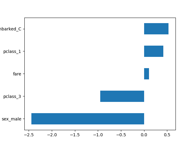
With the global configuration, all transformers output DataFrames. This allows us to easily plot the logistic regression coefficients with the corresponding feature names.
import pandas as pd
log_reg = clf[-1] coef = pd.Series(log_reg.coef_.ravel(), index=log_reg.feature_names_in_) _ = coef.sort_values().plot.barh()
In order to demonstrate the config_context functionality below, let us first reset transform_output to its default value.
When configuring the output type with config_context the configuration at the time when transform or fit_transform are called is what counts. Setting these only when you construct or fit the transformer has no effect.
StandardScaler()
In a Jupyter environment, please rerun this cell to show the HTML representation or trust the notebook. On GitHub, the HTML representation is unable to render, please try loading this page with nbviewer.org.
with config_context(transform_output="pandas"): # the output of transform will be a Pandas DataFrame X_test_scaled = scaler.transform(X_test[num_cols]) X_test_scaled.head()
| age | fare | |
|---|---|---|
| 391 | -0.044009 | -0.125325 |
| 701 | -0.880239 | -0.471468 |
| 591 | -1.716470 | -0.124794 |
| 1196 | -0.044009 | -0.456257 |
| 1049 | -0.671182 | -0.342893 |
outside of the context manager, the output will be a NumPy array
X_test_scaled = scaler.transform(X_test[num_cols]) X_test_scaled[:5]
array([[-0.04400864, -0.12532481], [-0.88023923, -0.47146783], [-1.71646982, -0.12479447], [-0.04400864, -0.45625688], [-0.67118158, -0.34289311]])
Total running time of the script: (0 minutes 0.143 seconds)
Related examples