Comparing Target Encoder with Other Encoders (original) (raw)
Note
Go to the endto download the full example code. or to run this example in your browser via JupyterLite or Binder
The TargetEncoder uses the value of the target to encode each categorical feature. In this example, we will compare three different approaches for handling categorical features: TargetEncoder,OrdinalEncoder, OneHotEncoder and dropping the category.
Note
fit(X, y).transform(X) does not equal fit_transform(X, y) because a cross fitting scheme is used in fit_transform for encoding. See theUser Guide. for details.
Authors: The scikit-learn developers
SPDX-License-Identifier: BSD-3-Clause
Loading Data from OpenML#
First, we load the wine reviews dataset, where the target is the points given be a reviewer:
from sklearn.datasets import fetch_openml
wine_reviews = fetch_openml(data_id=42074, as_frame=True)
df = wine_reviews.frame df.head()
| country | description | designation | points | price | province | region_1 | region_2 | variety | winery | |
|---|---|---|---|---|---|---|---|---|---|---|
| 0 | US | This tremendous 100% varietal wine hails from ... | Martha's Vineyard | 96 | 235.0 | California | Napa Valley | Napa | Cabernet Sauvignon | Heitz |
| 1 | Spain | Ripe aromas of fig, blackberry and cassis are ... | Carodorum Selección Especial Reserva | 96 | 110.0 | Northern Spain | Toro | NaN | Tinta de Toro | Bodega Carmen Rodríguez |
| 2 | US | Mac Watson honors the memory of a wine once ma... | Special Selected Late Harvest | 96 | 90.0 | California | Knights Valley | Sonoma | Sauvignon Blanc | Macauley |
| 3 | US | This spent 20 months in 30% new French oak, an... | Reserve | 96 | 65.0 | Oregon | Willamette Valley | Willamette Valley | Pinot Noir | Ponzi |
| 4 | France | This is the top wine from La Bégude, named aft... | La Brûlade | 95 | 66.0 | Provence | Bandol | NaN | Provence red blend | Domaine de la Bégude |
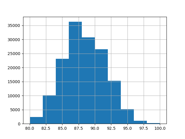
For this example, we use the following subset of numerical and categorical features in the data. The target are continuous values from 80 to 100:
numerical_features = ["price"] categorical_features = [ "country", "province", "region_1", "region_2", "variety", "winery", ] target_name = "points"
X = df[numerical_features + categorical_features] y = df[target_name]
_ = y.hist()
Training and Evaluating Pipelines with Different Encoders#
In this section, we will evaluate pipelines withHistGradientBoostingRegressor with different encoding strategies. First, we list out the encoders we will be using to preprocess the categorical features:
from sklearn.compose import ColumnTransformer from sklearn.preprocessing import OneHotEncoder, OrdinalEncoder, TargetEncoder
categorical_preprocessors = [ ("drop", "drop"), ("ordinal", OrdinalEncoder(handle_unknown="use_encoded_value", unknown_value=-1)), ( "one_hot", OneHotEncoder(handle_unknown="ignore", max_categories=20, sparse_output=False), ), ("target", TargetEncoder(target_type="continuous")), ]
Next, we evaluate the models using cross validation and record the results:
from sklearn.ensemble import HistGradientBoostingRegressor from sklearn.model_selection import cross_validate from sklearn.pipeline import make_pipeline
n_cv_folds = 3 max_iter = 20 results = []
def evaluate_model_and_store(name, pipe): result = cross_validate( pipe, X, y, scoring="neg_root_mean_squared_error", cv=n_cv_folds, return_train_score=True, ) rmse_test_score = -result["test_score"] rmse_train_score = -result["train_score"] results.append( { "preprocessor": name, "rmse_test_mean": rmse_test_score.mean(), "rmse_test_std": rmse_train_score.std(), "rmse_train_mean": rmse_train_score.mean(), "rmse_train_std": rmse_train_score.std(), } )
for name, categorical_preprocessor in categorical_preprocessors: preprocessor = ColumnTransformer( [ ("numerical", "passthrough", numerical_features), ("categorical", categorical_preprocessor, categorical_features), ] ) pipe = make_pipeline( preprocessor, HistGradientBoostingRegressor(random_state=0, max_iter=max_iter) ) evaluate_model_and_store(name, pipe)
Native Categorical Feature Support#
In this section, we build and evaluate a pipeline that uses native categorical feature support in HistGradientBoostingRegressor, which only supports up to 255 unique categories. In our dataset, the most of the categorical features have more than 255 unique categories:
n_unique_categories = df[categorical_features].nunique().sort_values(ascending=False) n_unique_categories
winery 14810 region_1 1236 variety 632 province 455 country 48 region_2 18 dtype: int64
To workaround the limitation above, we group the categorical features into low cardinality and high cardinality features. The high cardinality features will be target encoded and the low cardinality features will use the native categorical feature in gradient boosting.
high_cardinality_features = n_unique_categories[n_unique_categories > 255].index low_cardinality_features = n_unique_categories[n_unique_categories <= 255].index mixed_encoded_preprocessor = ColumnTransformer( [ ("numerical", "passthrough", numerical_features), ( "high_cardinality", TargetEncoder(target_type="continuous"), high_cardinality_features, ), ( "low_cardinality", OrdinalEncoder(handle_unknown="use_encoded_value", unknown_value=-1), low_cardinality_features, ), ], verbose_feature_names_out=False, )
The output of the of the preprocessor must be set to pandas so the
gradient boosting model can detect the low cardinality features.
mixed_encoded_preprocessor.set_output(transform="pandas") mixed_pipe = make_pipeline( mixed_encoded_preprocessor, HistGradientBoostingRegressor( random_state=0, max_iter=max_iter, categorical_features=low_cardinality_features ), ) mixed_pipe
Pipeline(steps=[('columntransformer', ColumnTransformer(transformers=[('numerical', 'passthrough', ['price']), ('high_cardinality', TargetEncoder(target_type='continuous'), Index(['winery', 'region_1', 'variety', 'province'], dtype='object')), ('low_cardinality', OrdinalEncoder(handle_unknown='use_encoded_value', unknown_value=-1), Index(['country', 'region_2'], dtype='object'))], verbose_feature_names_out=False)), ('histgradientboostingregressor', HistGradientBoostingRegressor(categorical_features=Index(['country', 'region_2'], dtype='object'), max_iter=20, random_state=0))])
Finally, we evaluate the pipeline using cross validation and record the results:
evaluate_model_and_store("mixed_target", mixed_pipe)
Plotting the Results#
In this section, we display the results by plotting the test and train scores:
import matplotlib.pyplot as plt import pandas as pd
results_df = ( pd.DataFrame(results).set_index("preprocessor").sort_values("rmse_test_mean") )
fig, (ax1, ax2) = plt.subplots( 1, 2, figsize=(12, 8), sharey=True, constrained_layout=True ) xticks = range(len(results_df)) name_to_color = dict( zip((r["preprocessor"] for r in results), ["C0", "C1", "C2", "C3", "C4"]) )
for subset, ax in zip(["test", "train"], [ax1, ax2]): mean, std = f"rmse_{subset}mean", f"rmse{subset}_std" data = results_df[[mean, std]].sort_values(mean) ax.bar( x=xticks, height=data[mean], yerr=data[std], width=0.9, color=[name_to_color[name] for name in data.index], ) ax.set( title=f"RMSE ({subset.title()})", xlabel="Encoding Scheme", xticks=xticks, xticklabels=data.index, )
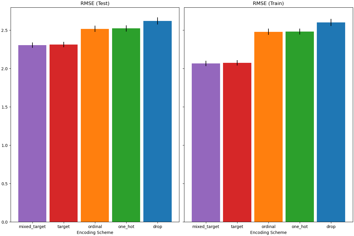
When evaluating the predictive performance on the test set, dropping the categories perform the worst and the target encoders performs the best. This can be explained as follows:
- Dropping the categorical features makes the pipeline less expressive and underfitting as a result;
- Due to the high cardinality and to reduce the training time, the one-hot encoding scheme uses
max_categories=20which prevents the features from expanding too much, which can result in underfitting. - If we had not set
max_categories=20, the one-hot encoding scheme would have likely made the pipeline overfitting as the number of features explodes with rare category occurrences that are correlated with the target by chance (on the training set only); - The ordinal encoding imposes an arbitrary order to the features which are then treated as numerical values by theHistGradientBoostingRegressor. Since this model groups numerical features in 256 bins per feature, many unrelated categories can be grouped together and as a result overall pipeline can underfit;
- When using the target encoder, the same binning happens, but since the encoded values are statistically ordered by marginal association with the target variable, the binning use by the HistGradientBoostingRegressormakes sense and leads to good results: the combination of smoothed target encoding and binning works as a good regularizing strategy against overfitting while not limiting the expressiveness of the pipeline too much.
Total running time of the script: (0 minutes 22.041 seconds)
Related examples