Understanding the decision tree structure (original) (raw)
Note
Go to the endto download the full example code. or to run this example in your browser via JupyterLite or Binder
The decision tree structure can be analysed to gain further insight on the relation between the features and the target to predict. In this example, we show how to retrieve:
- the binary tree structure;
- the depth of each node and whether or not it’s a leaf;
- the nodes that were reached by a sample using the
decision_pathmethod; - the leaf that was reached by a sample using the apply method;
- the rules that were used to predict a sample;
- the decision path shared by a group of samples.
Authors: The scikit-learn developers
SPDX-License-Identifier: BSD-3-Clause
import numpy as np from matplotlib import pyplot as plt
from sklearn import tree from sklearn.datasets import load_iris from sklearn.model_selection import train_test_split from sklearn.tree import DecisionTreeClassifier
Train tree classifier#
First, we fit a DecisionTreeClassifier using theload_iris dataset.
DecisionTreeClassifier(max_leaf_nodes=3, random_state=0)
In a Jupyter environment, please rerun this cell to show the HTML representation or trust the notebook. On GitHub, the HTML representation is unable to render, please try loading this page with nbviewer.org.
Tree structure#
The decision classifier has an attribute called tree_ which allows access to low level attributes such as node_count, the total number of nodes, and max_depth, the maximal depth of the tree. Thetree_.compute_node_depths() method computes the depth of each node in the tree. tree_ also stores the entire binary tree structure, represented as a number of parallel arrays. The i-th element of each array holds information about the node i. Node 0 is the tree’s root. Some of the arrays only apply to either leaves or split nodes. In this case the values of the nodes of the other type is arbitrary. For example, the arrays feature andthreshold only apply to split nodes. The values for leaf nodes in these arrays are therefore arbitrary.
Among these arrays, we have:
children_left[i]: id of the left child of nodeior -1 if leaf nodechildren_right[i]: id of the right child of nodeior -1 if leaf nodefeature[i]: feature used for splitting nodeithreshold[i]: threshold value at nodein_node_samples[i]: the number of training samples reaching nodeiimpurity[i]: the impurity at nodeiweighted_n_node_samples[i]: the weighted number of training samples reaching nodeivalue[i, j, k]: the summary of the training samples that reached node i for output j and class k (for regression tree, class is set to 1). See below for more information aboutvalue.
Using the arrays, we can traverse the tree structure to compute various properties. Below, we will compute the depth of each node and whether or not it is a leaf.
n_nodes = clf.tree_.node_count children_left = clf.tree_.children_left children_right = clf.tree_.children_right feature = clf.tree_.feature threshold = clf.tree_.threshold values = clf.tree_.value
node_depth = np.zeros(shape=n_nodes, dtype=np.int64)
is_leaves = np.zeros(shape=n_nodes, dtype=bool)
stack = [(0, 0)] # start with the root node id (0) and its depth (0)
while len(stack) > 0:
# pop ensures each node is only visited once
node_id, depth = stack.pop()
node_depth[node_id] = depth
# If the left and right child of a node is not the same we have a split
# node
is_split_node = children_left[node_id] != children_right[node_id]
# If a split node, append left and right children and depth to `stack`
# so we can loop through them
if is_split_node:
    stack.append((children_left[node_id], depth + 1))
    stack.append((children_right[node_id], depth + 1))
else:
    is_leaves[node_id] = True
print( "The binary tree structure has {n} nodes and has " "the following tree structure:\n".format(n=n_nodes) ) for i in range(n_nodes): if is_leaves[i]: print( "{space}node={node} is a leaf node with value={value}.".format( space=node_depth[i] * "\t", node=i, value=np.around(values[i], 3) ) ) else: print( "{space}node={node} is a split node with value={value}: " "go to node {left} if X[:, {feature}] <= {threshold} " "else to node {right}.".format( space=node_depth[i] * "\t", node=i, left=children_left[i], feature=feature[i], threshold=threshold[i], right=children_right[i], value=np.around(values[i], 3), ) )
The binary tree structure has 5 nodes and has the following tree structure:
node=0 is a split node with value=[[0.33 0.304 0.366]]: go to node 1 if X[:, 3] <= 0.800000011920929 else to node 2. node=1 is a leaf node with value=[[1. 0. 0.]]. node=2 is a split node with value=[[0. 0.453 0.547]]: go to node 3 if X[:, 2] <= 4.950000047683716 else to node 4. node=3 is a leaf node with value=[[0. 0.917 0.083]]. node=4 is a leaf node with value=[[0. 0.026 0.974]].
What is the values array used here?#
The tree_.value array is a 3D array of shape [n_nodes, n_classes, n_outputs] which provides the proportion of samples reaching a node for each class and for each output. Each node has a value array which is the proportion of weighted samples reaching this node for each output and class with respect to the parent node.
One could convert this to the absolute weighted number of samples reaching a node, by multiplying this number by tree_.weighted_n_node_samples[node_idx] for the given node. Note sample weights are not used in this example, so the weighted number of samples is the number of samples reaching the node because each sample has a weight of 1 by default.
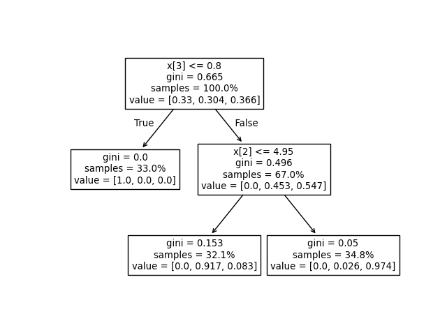
For example, in the above tree built on the iris dataset, the root node hasvalue = [0.33, 0.304, 0.366] indicating there are 33% of class 0 samples, 30.4% of class 1 samples, and 36.6% of class 2 samples at the root node. One can convert this to the absolute number of samples by multiplying by the number of samples reaching the root node, which is tree_.weighted_n_node_samples[0]. Then the root node has value = [37, 34, 41], indicating there are 37 samples of class 0, 34 samples of class 1, and 41 samples of class 2 at the root node.
Traversing the tree, the samples are split and as a result, the value array reaching each node changes. The left child of the root node has value = [1., 0, 0](or value = [37, 0, 0] when converted to the absolute number of samples) because all 37 samples in the left child node are from class 0.
Note: In this example, n_outputs=1, but the tree classifier can also handle multi-output problems. The value array at each node would just be a 2D array instead.
We can compare the above output to the plot of the decision tree. Here, we show the proportions of samples of each class that reach each node corresponding to the actual elements of tree_.value array.
Decision path#
We can also retrieve the decision path of samples of interest. Thedecision_path method outputs an indicator matrix that allows us to retrieve the nodes the samples of interest traverse through. A non zero element in the indicator matrix at position (i, j) indicates that the sample i goes through the node j. Or, for one sample i, the positions of the non zero elements in row i of the indicator matrix designate the ids of the nodes that sample goes through.
The leaf ids reached by samples of interest can be obtained with theapply method. This returns an array of the node ids of the leaves reached by each sample of interest. Using the leaf ids and thedecision_path we can obtain the splitting conditions that were used to predict a sample or a group of samples. First, let’s do it for one sample. Note that node_index is a sparse matrix.
node_indicator = clf.decision_path(X_test) leaf_id = clf.apply(X_test)
sample_id = 0
obtain ids of the nodes sample_id goes through, i.e., row sample_id
node_index = node_indicator.indices[ node_indicator.indptr[sample_id] : node_indicator.indptr[sample_id + 1] ]
print("Rules used to predict sample {id}:\n".format(id=sample_id)) for node_id in node_index: # continue to the next node if it is a leaf node if leaf_id[sample_id] == node_id: continue
# check if value of the split feature for sample 0 is below threshold
if X_test[sample_id, feature[node_id]] <= threshold[node_id]:
    threshold_sign = "<="
else:
    threshold_sign = ">"

print(
    "decision node {node} : (X_test[{sample}, {feature}] = {value}) "
    "{inequality} {threshold})".format(
        node=node_id,
        sample=sample_id,
        feature=feature[node_id],
        value=X_test[sample_id, feature[node_id]],
        inequality=threshold_sign,
        threshold=threshold[node_id],
    )
)
Rules used to predict sample 0:
decision node 0 : (X_test[0, 3] = 2.4) > 0.800000011920929) decision node 2 : (X_test[0, 2] = 5.1) > 4.950000047683716)
For a group of samples, we can determine the common nodes the samples go through.
sample_ids = [0, 1]
boolean array indicating the nodes both samples go through
common_nodes = node_indicator.toarray()[sample_ids].sum(axis=0) == len(sample_ids)
obtain node ids using position in array
common_node_id = np.arange(n_nodes)[common_nodes]
print( "\nThe following samples {samples} share the node(s) {nodes} in the tree.".format( samples=sample_ids, nodes=common_node_id ) ) print("This is {prop}% of all nodes.".format(prop=100 * len(common_node_id) / n_nodes))
The following samples [0, 1] share the node(s) [0 2] in the tree. This is 40.0% of all nodes.
Total running time of the script: (0 minutes 0.076 seconds)
Related examples