Use Bayesian Optimization in Custom Training Experiments - MATLAB & Simulink (original) (raw)

Main Content

This example shows how to use Bayesian optimization to find optimal hyperparameter values for custom training experiments in Experiment Manager. Instead of sweeping hyperparameters, you specify a range of values for each hyperparameter and select a metric to optimize. Experiment Manager searches for a combination of hyperparameters that optimizes that metric.

In this example, you train a network to classify images of handwritten digits using a custom learning rate schedule. The experiment uses Bayesian optimization to find the type of schedule and the combination of hyperparameters that maximizes the validation accuracy. For more information on using a custom learning rate schedule, see Train Network Using Custom Training Loop and Piecewise Learn Rate Schedule.

Alternatively, you can find optimal hyperparameter values programmatically by calling the bayesopt function. For more information, see Deep Learning Using Bayesian Optimization.

Open Experiment

First, open the example. Experiment Manager loads a project with a preconfigured experiment that you can inspect and run. To open the experiment, in the Experiment Browser pane, double-click BayesOptExperiment.

Custom training experiments consist of a description, a table of hyperparameters, and a training function. Experiments that use Bayesian optimization include additional options to limit the duration of the experiment. For more information, see Train Network Using Custom Training Loop and Display Visualization.

The Description field contains a textual description of the experiment. For this example, the description is:

Classification of digits, using two custom learning rate schedules:

decay - Use the learning rate p(t) = p(0)/(1+kt), where t is the iteration number and k is DecayRate.
piecewise - Multiply the learning rate by DropFactor every 100 iterations.

The Hyperparameters section specifies the strategy and hyperparameter options to use for the experiment. For each hyperparameter, you can specify these options:

Range — Enter a two-element vector that gives the lower bound and upper bound of a real- or integer-valued hyperparameter, or a string array or cell array that lists the possible values of a categorical hyperparameter.
Type — Select real for a real-valued hyperparameter, integer for an integer-valued hyperparameter, or categorical for a categorical hyperparameter.
Transform — Select none to use no transform or log to use a logarithmic transform. When you select log, the hyperparameter values must be positive. With this setting, the Bayesian optimization algorithm models the hyperparameter on a logarithmic scale.

When you run the experiment, Experiment Manager searches for the best combination of hyperparameters. Each trial in the experiment uses a new combination of hyperparameter values based on the results of the previous trials. This example uses the hyperparameters Schedule, InitialLearnRate, DecayRate, and DropFactor to specify the custom learning rate schedule used for training. The options for Schedule are:

decay — For each iteration, use the time-based learning rate $\rho_t = \frac{\rho_0}{1+kt}$ , where is the iteration number, $\rho_0$ is the initial learning rate specified by InitialLearnRate, and is the decay rate specified by DecayRate. This option ignores the value of the hyperparameter DropFactor.
piecewise — Start with the initial learning rate specified by InitialLearnRate and periodically drop the learning rate by multiplying by the drop factor specified by DropFactor. In this example, the learning rate drops every 100 iterations. This option ignores the value of the hyperparameter DecayRate.

The experiment models InitialLearnRate and DecayRate on a logarithmic scale because the range of values for these hyperparameters spans several orders of magnitude, from 0.001 to 0.1. In contrast, the values for DropFactor range from 0.1 to 0.9, so the experiment models DropFactor on a linear scale.

Under Bayesian Optimization Options, you can specify the duration of the experiment by entering the maximum time in seconds and the maximum number of trials to run. To best use the power of Bayesian optimization, perform at least 30 objective function evaluations.

The Training Function section specifies a function that defines the training data, network architecture, training options, and training procedure used by the experiment. To open this function in MATLAB® Editor, click Edit. The code for the function also appears in Training Function. The input to the training function is a structure with fields from the hyperparameter table and an experiments.Monitor object that you can use to track the progress of the training, record values of the metrics used by the training, and produce training plots. The function returns a structure that contains the trained network, the training loss, the validation accuracy, and the execution environment used for training. Experiment Manager saves this output so you can export it to the MATLAB workspace when the training is complete. The training function has these sections:

Initialize Output sets the initial value of the network, loss, and accuracy to empty arrays to indicate that the training has not started. The experiment sets the execution environment to "auto", so it trains the network on a GPU if one is available. Using a GPU requires Parallel Computing Toolbox™ and a supported GPU device. For more information, see GPU Computing Requirements (Parallel Computing Toolbox).

output.trainedNet = []; output.trainingInfo.loss = []; output.trainingInfo.accuracy = []; output.executionEnvironment = "auto";

Load Training Data defines the training and validation data for the experiment as augmented image datastores using the Digits data set. For each image in the training set, the experiment applies a random translation of up to 5 pixels on the horizontal and vertical axes. For more information on this data set, see Image Data Sets.

dataFolder = fullfile(toolboxdir('nnet'), ... 'nndemos','nndatasets','DigitDataset'); imds = imageDatastore(dataFolder, ... IncludeSubfolders=true, ... LabelSource="foldernames"); [imdsTrain,imdsValidation] = splitEachLabel(imds,0.9,"randomize");

inputSize = [28 28 1]; pixelRange = [-5 5]; imageAugmenter = imageDataAugmenter( ... RandXTranslation = pixelRange, ... RandYTranslation = pixelRange); augimdsTrain = augmentedImageDatastore(inputSize(1:2),imdsTrain, ... DataAugmentation = imageAugmenter); augimdsValidation = augmentedImageDatastore(inputSize(1:2),imdsValidation); classes = categories(imdsTrain.Labels); numClasses = numel(classes);

Define Network Architecture defines the architecture for the image classification network. To train the network with a custom training loop and enable automatic differentiation, the training function converts the layer graph to a dlnetwork object.

layers = [ imageInputLayer(inputSize,Normalization="none") convolution2dLayer(5,20) batchNormalizationLayer() reluLayer() convolution2dLayer(3,20,Padding="same") batchNormalizationLayer() reluLayer() convolution2dLayer(3,20,Padding="same") batchNormalizationLayer() reluLayer() fullyConnectedLayer(numClasses) softmaxLayer()];

lgraph = layerGraph(layers); net = dlnetwork(lgraph);

Specify Training Options defines the training options used by the experiment. In this example, Experiment Manager trains the networks with a mini-batch size of 128 for 10 epochs using the custom learning rate schedule defined by the hyperparameters.

numEpochs = 10; miniBatchSize = 128; momentum = 0.9;

learnRateSchedule = params.Schedule; initialLearnRate = params.InitialLearnRate; learnRateDecay = params.DecayRate; learnRateDropFactor = params.DropFactor; learnRateDropPeriod = 100; learnRate = initialLearnRate;

Train Model defines the custom training loop used by the experiment. The custom training loop uses minibatchqueue to process and manage the mini-batches of images. For each mini-batch, the minibatchqueue object converts the labels to one-hot encoded variables and formats the image data with the dimension labels "SSCB" (spatial, spatial, channel, batch). By default, the minibatchqueue object converts the data to dlarray objects with underlying type single. If you train on a GPU, the data is converted to gpuArray (Parallel Computing Toolbox) objects. For each epoch, the custom training loop shuffles the datastore, loops over mini-batches of data, and evaluates the model loss, gradients, and state. Then, the training function determines the learning rate for the selected schedule and updates the network parameters. After each iteration of the custom training loop, the training function computes the validation accuracy, saves the trained network, and updates the training progress.

monitor.Metrics = ["LearnRate" "TrainingLoss" "ValidationAccuracy"]; monitor.XLabel = "Iteration";

mbq = minibatchqueue(augimdsTrain,... MiniBatchSize=miniBatchSize,... MiniBatchFcn=@preprocessMiniBatch,... MiniBatchFormat=["SSCB",""],... OutputEnvironment=output.executionEnvironment);

iteration = 0; velocity = []; recordMetrics(monitor,iteration,ValidationAccuracy=0);

for epoch = 1:numEpochs shuffle(mbq);

while hasdata(mbq)
    iteration = iteration + 1;

    [X,Y] = next(mbq);

    [loss,gradients,state] = dlfeval(@modelLoss,net,X,Y);
    loss = double(gather(extractdata(loss)));
    net.State = state;

    switch learnRateSchedule
        case "decay"
            learnRate = initialLearnRate/(1 + learnRateDecay*iteration);
        case "piecewise"
            if mod(iteration,learnRateDropPeriod) == 0
                learnRate = learnRate*learnRateDropFactor;
            end
    end

    recordMetrics(monitor,iteration, ...
        LearnRate=learnRate, ...
        TrainingLoss=loss);
    output.trainingInfo.loss = [output.trainingInfo.loss; iteration loss];
    [net,velocity] = sgdmupdate(net,gradients,velocity,learnRate,momentum);

    if monitor.Stop
        return;
    end
end

numOutputs = 1;
mbqTest = minibatchqueue(augimdsValidation,numOutputs, ...
    MiniBatchSize=miniBatchSize, ...
    MiniBatchFcn=@preprocessMiniBatchPredictors, ...
    MiniBatchFormat="SSCB");
predictedLabels = modelPredictions(net,mbqTest,classes);
trueLabels = imdsValidation.Labels;
accuracy = mean(predictedLabels == trueLabels)*100.0;

output.trainedNet = net;
monitor.Progress = (epoch*100.0)/numEpochs;
recordMetrics(monitor,iteration, ...
    ValidationAccuracy=accuracy);
output.trainingInfo.accuracy = [output.trainingInfo.accuracy; iteration accuracy];

end

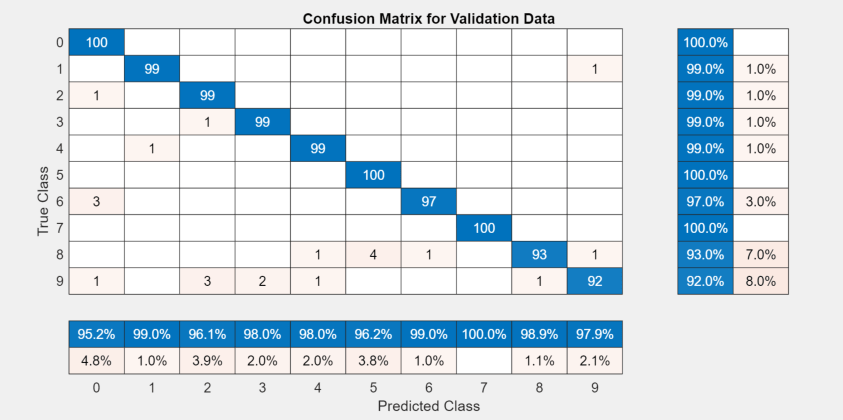
Plot Confusion Matrix calls the confusionchart function to create the confusion matrix for the validation data. When the training is complete, the Review Results gallery in the toolstrip displays a button for the confusion matrix. The Name property of the figure specifies the name of the button. You can click the button to display the confusion matrix in the Visualizations pane.

figure(Name="Confusion Matrix") confusionchart(trueLabels,predictedLabels, ... ColumnSummary="column-normalized", ... RowSummary="row-normalized", ... Title="Confusion Matrix for Validation Data");

In the Metrics section, the Optimize and Direction fields indicate the metric that the Bayesian optimization algorithm uses as an objective function. For this experiment, Experiment Manager seeks to maximize the value of the validation accuracy.

Run Experiment

When you run the experiment, Experiment Manager trains the network defined by the training function multiple times. Each trial uses a different combination of hyperparameter values.

Training can take some time. To limit the duration of the experiment, you can modify the Bayesian Optimization Options by reducing the maximum running time or the maximum number of trials. However, running fewer than 30 trials can prevent the Bayesian optimization algorithm from converging to an optimal set of hyperparameters.

By default, Experiment Manager runs one trial at a time. If you have Parallel Computing Toolbox, you can run multiple trials at the same time or offload your experiment as a batch job in a cluster:

To run one trial of the experiment at a time, on the Experiment Manager toolstrip, set Mode to Sequential and click Run.
To run multiple trials at the same time, set Mode to Simultaneous and click Run. If there is no current parallel pool, Experiment Manager starts one using the default cluster profile. Experiment Manager then runs as many simultaneous trials as there are workers in your parallel pool. For best results, before you run your experiment, start a parallel pool with as many workers as GPUs. For more information, see Run Experiments in Parallel and GPU Computing Requirements (Parallel Computing Toolbox).
To offload the experiment as a batch job, set Mode to Batch Sequential or Batch Simultaneous, specify your cluster and pool size, and click Run. For more information, see Offload Experiments as Batch Jobs to a Cluster.

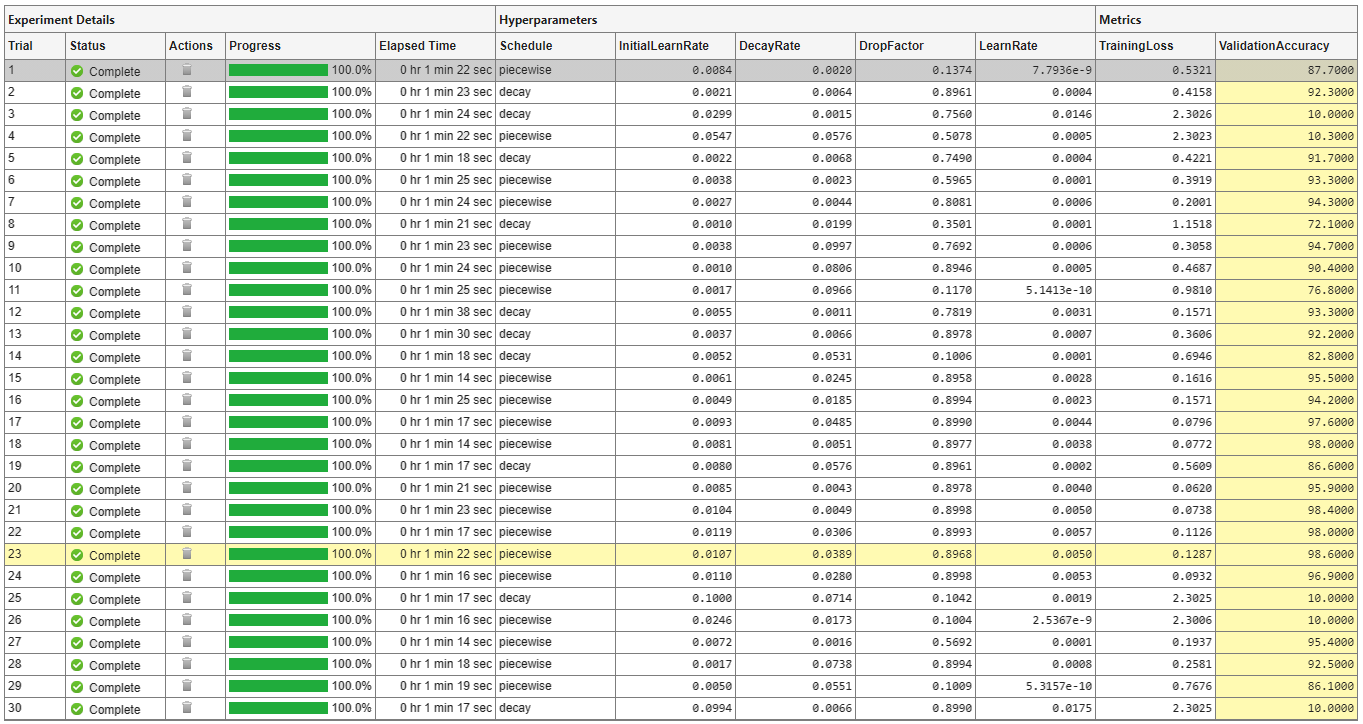
A table of results displays the training loss and validation accuracy for each trial. Experiment Manager highlights the trial with the optimal value for the selected metric. For example, in this experiment, the 23rd trial produces the greatest validation accuracy.

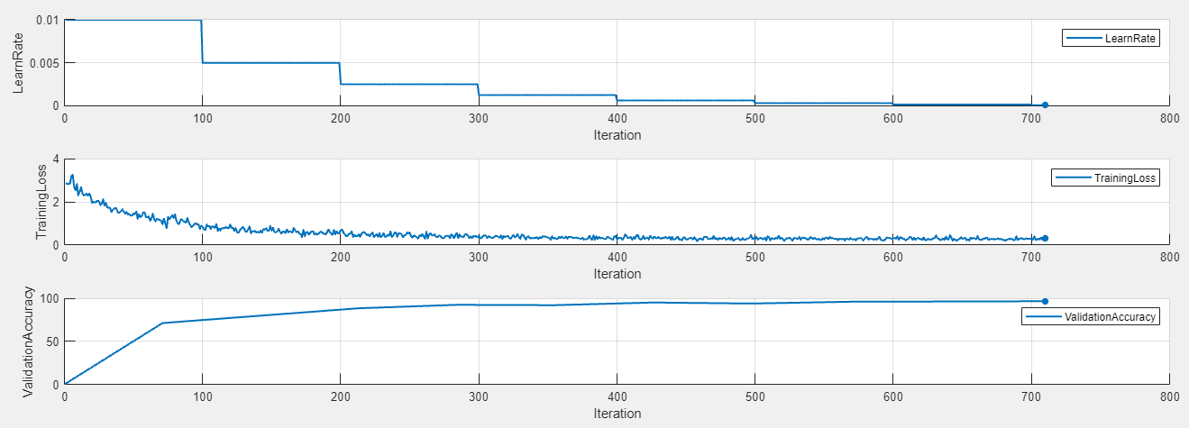
To display the training plot and track the progress of each trial while the experiment is running, under Review Results, click Training Plot. The training plot shows the learning rate, training loss, and validation accuracy for each trial. For example, this training plot is for a trial that uses a piecewise learning rate schedule.

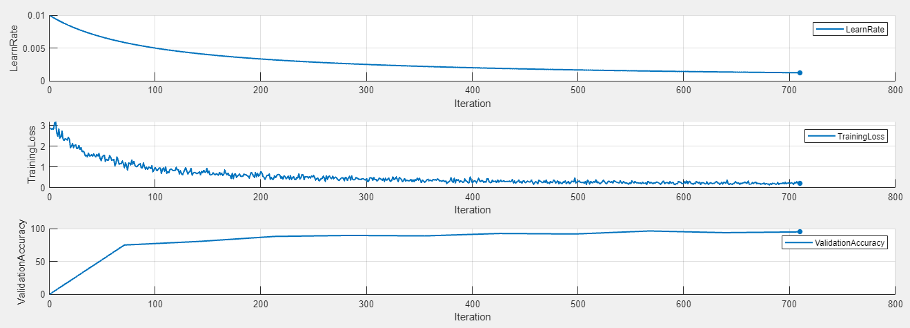
In contrast, this training plot is for a trial that uses a time-based decay learning rate schedule.

Evaluate Results

To display the confusion matrix for the best trial in your experiment, select the row in the results table with the highest validation accuracy. Then, under Review Results, click Confusion Matrix.

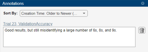
To record observations about the results of your experiment, add an annotation:

In the results table, right-click the ValidationAccuracy cell for the best trial.
Select Add Annotation.
In the Annotations pane, enter your observations in the text box.

Close Experiment

In the Experiment Browser pane, right-click DigitCustomLearningRateScheduleProject and select Close Project. Experiment Manager closes the experiment and results contained in the project.

Training Function

This function specifies the training data, network architecture, training options, and training procedure used by the experiment. The input to this function is a structure with fields from the hyperparameter table and an experiments.Monitor object that you can use to track the progress of the training, record values of the metrics used by the training, and produce training plots. The function returns a structure that contains the trained network, the training loss, the validation accuracy, and the execution environment used for training. Experiment Manager saves this output so you can export it to the MATLAB workspace when the training is complete.

function output = BayesOptExperiment_training(params,monitor)

Initialize Output

output.trainedNet = []; output.trainingInfo.loss = []; output.trainingInfo.accuracy = []; output.executionEnvironment = "auto";

Load Training Data

Define Network Architecture

lgraph = layerGraph(layers); net = dlnetwork(lgraph);

Specify Training Options

numEpochs = 10; miniBatchSize = 128; momentum = 0.9;

Train Model

monitor.Metrics = ["LearnRate" "TrainingLoss" "ValidationAccuracy"]; monitor.XLabel = "Iteration";

mbq = minibatchqueue(augimdsTrain,... MiniBatchSize=miniBatchSize,... MiniBatchFcn=@preprocessMiniBatch,... MiniBatchFormat=["SSCB",""],... OutputEnvironment=output.executionEnvironment);

iteration = 0; velocity = []; recordMetrics(monitor,iteration,ValidationAccuracy=0);

for epoch = 1:numEpochs shuffle(mbq);

while hasdata(mbq)
    iteration = iteration + 1;

    [X,Y] = next(mbq);

    [loss,gradients,state] = dlfeval(@modelLoss,net,X,Y);
    loss = double(gather(extractdata(loss)));
    net.State = state;

    switch learnRateSchedule
        case "decay"
            learnRate = initialLearnRate/(1 + learnRateDecay*iteration);
        case "piecewise"
            if mod(iteration,learnRateDropPeriod) == 0
                learnRate = learnRate*learnRateDropFactor;
            end
    end

    recordMetrics(monitor,iteration, ...
        LearnRate=learnRate, ...
        TrainingLoss=loss);
    output.trainingInfo.loss = [output.trainingInfo.loss; iteration loss];
    [net,velocity] = sgdmupdate(net,gradients,velocity,learnRate,momentum);

    if monitor.Stop
        return;
    end
end

numOutputs = 1;
mbqTest = minibatchqueue(augimdsValidation,numOutputs, ...
    MiniBatchSize=miniBatchSize, ...
    MiniBatchFcn=@preprocessMiniBatchPredictors, ...
    MiniBatchFormat="SSCB");
predictedLabels = modelPredictions(net,mbqTest,classes);
trueLabels = imdsValidation.Labels;
accuracy = mean(predictedLabels == trueLabels)*100.0;

output.trainedNet = net;
monitor.Progress = (epoch*100.0)/numEpochs;
recordMetrics(monitor,iteration, ...
    ValidationAccuracy=accuracy);
output.trainingInfo.accuracy = [output.trainingInfo.accuracy; iteration accuracy];

end

Plot Confusion Matrix

figure(Name="Confusion Matrix") confusionchart(trueLabels,predictedLabels, ... ColumnSummary="column-normalized", ... RowSummary="row-normalized", ... Title="Confusion Matrix for Validation Data");

Helper Functions

The modelLoss function takes a dlnetwork object net and a mini-batch of input data X with corresponding labels Y. The function returns the gradients of the loss with respect to the learnable parameters in net, the network state, and the loss. To compute the gradients automatically, the function calls the dlgradient function.

function [loss,gradients,state] = modelLoss(net,X,Y) [YPred,state] = forward(net,X); loss = crossentropy(YPred,Y); gradients = dlgradient(loss,net.Learnables); end

The modelPredictions function takes a dlnetwork object net, a minibatchqueue object mbq, and the network classes. The function computes the model predictions by iterating over the data in the minibatchqueue object. The function uses the onehotdecode function to find the predicted class with the highest score.

function predictions = modelPredictions(net,mbq,classes) predictions = []; while hasdata(mbq) XTest = next(mbq); YPred = predict(net,XTest); YPred = onehotdecode(YPred,classes,1)'; predictions = [predictions; YPred]; end end

The preprocessMiniBatch function preprocesses a mini-batch of predictors and labels using these steps:

Preprocess the images using the preprocessMiniBatchPredictors function.
Extract the label data from the incoming cell array and concatenate the data into a categorical array along the second dimension.
One-hot encode the categorical labels into numeric arrays. Encoding into the first dimension produces an encoded array that matches the shape of the network output.

function [X,Y] = preprocessMiniBatch(XCell,YCell) X = preprocessMiniBatchPredictors(XCell); Y = cat(2,YCell{1:end}); Y = onehotencode(Y,1); end

The preprocessMiniBatchPredictors function preprocesses a mini-batch of predictors by extracting the image data from the input cell array and concatenating the data into a numeric array.

function X = preprocessMiniBatchPredictors(XCell) X = cat(4,XCell{1:end}); end

Use Bayesian Optimization in Custom Training Experiments - MATLAB & Simulink (original) (raw)

Open Experiment

Run Experiment

Evaluate Results

Close Experiment

Training Function

Helper Functions

See Also

Apps

Objects

Functions

Use Bayesian Optimization in Custom Training Experiments - MATLAB & Simulink (original) (raw)

Open Experiment

Run Experiment

Evaluate Results

Close Experiment

Training Function

Helper Functions

See Also

Apps

Objects

Functions

Related Topics