Tune Experiment Hyperparameters by Using Bayesian Optimization - MATLAB & Simulink (original) (raw)
Main Content
This example shows how to use Bayesian optimization in Experiment Manager to find optimal network hyperparameters and training options for convolutional neural networks. Bayesian optimization provides an alternative strategy to sweeping hyperparameters in an experiment. You specify a range of values for each hyperparameter and select a metric to optimize, and Experiment Manager searches for a combination of hyperparameters that optimizes your selected metric. Bayesian optimization requires Statistics and Machine Learning Toolbox™.
In this example, you train a network to classify images from the CIFAR-10 data set. The experiment uses Bayesian optimization to find the combination of hyperparameters that minimizes a custom metric function. The hyperparameters include options of the training algorithm, as well as parameters of the network architecture itself. The custom metric function determines the classification error on a randomly chosen test set. For more information on defining custom metrics in Experiment Manager, see Evaluate Deep Learning Experiments by Using Metric Functions.
Alternatively, you can find optimal hyperparameter values programmatically by calling the bayesopt function. For more information, see Deep Learning Using Bayesian Optimization.
Open Experiment
First, open the example. Experiment Manager loads a project with a preconfigured experiment that you can inspect and run. To open the experiment, in the Experiment Browser pane, double-click BayesOptExperiment.
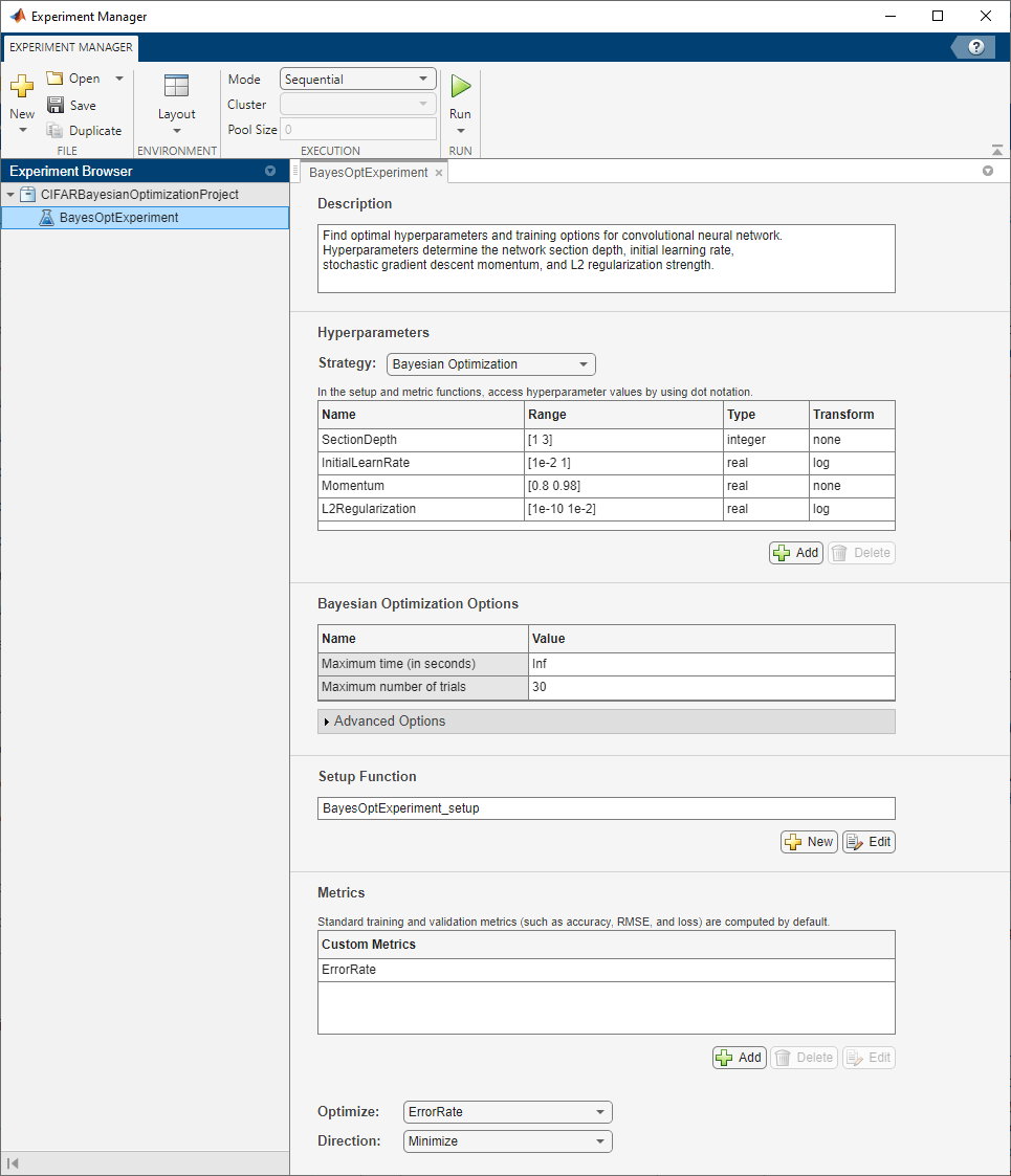
Built-in training experiments consist of a description, a table of hyperparameters, a setup function, and a collection of metric functions to evaluate the results of the experiment. Experiments that use Bayesian optimization include additional options to limit the duration of the experiment. For more information, see Train Network Using trainnet and Display Custom Metrics.
The Description field contains a textual description of the experiment. For this example, the description is:
Find optimal hyperparameters and training options for convolutional neural network. Hyperparameters determine the network section depth, initial learning rate, stochastic gradient descent momentum, and L2 regularization strength.
The Hyperparameters section specifies the strategy and hyperparameter options to use for the experiment. For each hyperparameter, you can specify these options:
- Range — Enter a two-element vector that gives the lower bound and upper bound of a real- or integer-valued hyperparameter, or a string array or cell array that lists the possible values of a categorical hyperparameter.
- Type — Select
realfor a real-valued hyperparameter,integerfor an integer-valued hyperparameter, orcategoricalfor a categorical hyperparameter. - Transform — Select
noneto use no transform orlogto use a logarithmic transform. When you selectlog, the hyperparameter values must be positive. With this setting, the Bayesian optimization algorithm models the hyperparameter on a logarithmic scale.
When you run the experiment, Experiment Manager searches for the best combination of hyperparameters. Each trial in the experiment uses a new combination of hyperparameter values based on the results of the previous trials. This example uses these hyperparameters:
SectionDepth— This parameter controls the depth of the network. The total number of layers in the network is9*SectionDepth+7. In the experiment setup function, the number of convolutional filters in each layer is proportional to1/sqrt(SectionDepth), so the number of parameters and the required amount of computation for each iteration are roughly the same for different section depths.InitialLearnRate— If the learning rate is too low, then training takes a long time. If the learning rate is too high, then training can reach a suboptimal result or diverge. The best learning rate can depend on your data as well as the network you are training.Momentum— Stochastic gradient descent momentum adds inertia to the parameter updates by having the current update contain a contribution proportional to the update in the previous iteration. The inertial effect results in smoother parameter updates and a reduction of the noise inherent to stochastic gradient descent.L2Regularization— Use L2 regularization to prevent overfitting. Search the space of regularization strength to find a good value. Data augmentation and batch normalization also help regularize the network.
Under Bayesian Optimization Options, you can specify the duration of the experiment by entering the maximum time (in seconds) and the maximum number of trials to run. To best use the power of Bayesian optimization, perform at least 30 objective function evaluations.
The Setup Function section specifies a function that configures the training data, network architecture, and training options for the experiment. To open this function in MATLAB® Editor, click Edit. The code for the function also appears in Setup Function. The input to the setup function is a structure with fields from the hyperparameter table. The function returns three outputs that you use to train a network for image classification problems. In this example, the setup function has these sections:
- Load Training Data downloads and extracts images and labels from the CIFAR-10 data set. The data set is about 175 MB. Depending on your internet connection, the download process can take some time. For the training data, this example creates an augmentedImageDatastore by applying random translations and horizontal reflections. Data augmentation helps prevent the network from overfitting and memorizing the exact details of the training images. To enable network validation, the example uses 5000 images with no augmentation. For more information on this data set, see Image Data Sets.
datadir = tempdir; downloadCIFARData(datadir);
[XTrain,YTrain,XTest,YTest] = loadCIFARData(datadir);
idx = randperm(numel(YTest),5000); XValidation = XTest(:,:,:,idx); YValidation = YTest(idx);
imageSize = [32 32 3];
pixelRange = [-4 4]; imageAugmenter = imageDataAugmenter( ... RandXReflection=true, ... RandXTranslation=pixelRange, ... RandYTranslation=pixelRange); augimdsTrain = augmentedImageDatastore(imageSize,XTrain,YTrain, ... DataAugmentation=imageAugmenter);
- Define Network Architecture defines the architecture for a convolutional neural network for deep learning classification. In this example, the network to train has three blocks produced by the helper function
convBlock. To view the code for this function, see Create Block of Convolutional Layers. Each block containsSectionDepthidentical convolutional layers. Each convolutional layer is followed by a batch normalization layer and a ReLU layer. The convolutional layers have added padding so that their spatial output size is always the same as the input size. Between the blocks, max pooling layers downsample the spatial dimensions by a factor of two. To ensure that the amount of computation required in each convolutional layer is roughly the same, the number of filters increases by a factor of two from one section to the next. The number of filters in each convolutional layer is proportional to1/sqrt(SectionDepth), so that networks of different depths have roughly the same number of parameters and require about the same amount of computation per iteration.
numClasses = numel(unique(YTrain)); numF = round(16/sqrt(params.SectionDepth));
layers = [ imageInputLayer(imageSize)
convBlock(3,numF,params.SectionDepth)
maxPooling2dLayer(3,Stride=2,Padding="same")

convBlock(3,2*numF,params.SectionDepth)
maxPooling2dLayer(3,Stride=2,Padding="same")

convBlock(3,4*numF,params.SectionDepth)
averagePooling2dLayer(8)

fullyConnectedLayer(numClasses)
softmaxLayer
classificationLayer];- Specify Training Options defines a trainingOptions object for the experiment using the values for the training options
InitialLearnRate,Momentum, andL2Regularizationgenerated by the Bayesian optimization algorithm. The example trains the network for a fixed number of epochs, validating once per epoch and lowering the learning rate by a factor of 10 during the last epochs to reduce the noise of the parameter updates and allow the network parameters to settle down closer to a minimum of the loss function.
miniBatchSize = 256; validationFrequency = floor(numel(YTrain)/miniBatchSize);
options = trainingOptions("sgdm", ... InitialLearnRate=params.InitialLearnRate, ... Momentum=params.Momentum, ... MaxEpochs=60, ... LearnRateSchedule="piecewise", ... LearnRateDropPeriod=40, ... LearnRateDropFactor=0.1, ... MiniBatchSize=miniBatchSize, ... L2Regularization=params.L2Regularization, ... Shuffle="every-epoch", ... Verbose=false, ... ValidationData={XValidation,YValidation}, ... ValidationFrequency=validationFrequency);
The Metrics section specifies optional functions that evaluate the results of the experiment. Experiment Manager evaluates these functions each time it finishes training the network. This example includes the custom metric function ErrorRate. This function selects 5000 test images and labels at random, evaluates the trained network on these images, and calculates the proportion of images that the network misclassifies. To open this function in MATLAB Editor, select the name of the metric function and click Edit. The code for the function also appears in Compute Error Rate.
The Optimize and Direction fields indicate the metric that the Bayesian optimization algorithm uses as an objective function. For this experiment, Experiment Manager seeks to minimize the value of the ErrorRate metric.
Run Experiment
When you run the experiment, Experiment Manager searches for the best combination of hyperparameters with respect to the chosen metric. Each trial in the experiment uses a new combination of hyperparameter values based on the results of the previous trials.
Training can take some time. To limit the duration of the experiment, you can modify the Bayesian Optimization Options by reducing the maximum running time or the maximum number of trials. However, note that running fewer than 30 trials can prevent the Bayesian optimization algorithm from converging to an optimal set of hyperparameters.
By default, Experiment Manager runs one trial at a time. If you have Parallel Computing Toolbox™, you can run multiple trials at the same time or offload your experiment as a batch job in a cluster:
- To run one trial of the experiment at a time, on the Experiment Manager toolstrip, set Mode to
Sequentialand click Run. - To run multiple trials at the same time, set Mode to
Simultaneousand click Run. If there is no current parallel pool, Experiment Manager starts one using the default cluster profile. Experiment Manager then runs as many simultaneous trials as there are workers in your parallel pool. For best results, before you run your experiment, start a parallel pool with as many workers as GPUs. For more information, see Run Experiments in Parallel and GPU Computing Requirements (Parallel Computing Toolbox). - To offload the experiment as a batch job, set Mode to
Batch SequentialorBatch Simultaneous, specify your cluster and pool size, and click Run. For more information, see Offload Experiments as Batch Jobs to a Cluster.
A table of results displays the metric function values for each trial. Experiment Manager highlights the trial with the optimal value for the selected metric. For example, in this experiment, the fifth trial produces the smallest error rate.

To determine the trial that optimizes the selected metric, Experiment Manager uses the best point criterion "min-observed". For more information, see Bayesian Optimization Algorithm (Statistics and Machine Learning Toolbox) and bestPoint (Statistics and Machine Learning Toolbox).
Evaluate Results
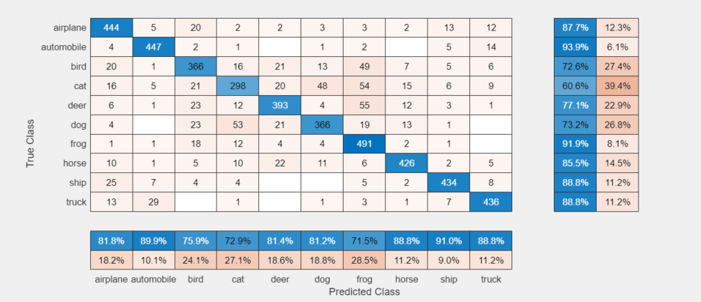
To display the confusion matrix for the best trial in your experiment, select the row in the results table with the lowest error rate. Then, under Review Results, click Validation Data.
To perform additional computations, export the trained network to the workspace:
- On the Experiment Manager toolstrip, click Export > Trained Network.
- In the dialog window, enter the name of a workspace variable for the exported network. The default name is
trainedNetwork. - In the MATLAB Command Window, use the exported network as the input to the helper function
testSummary:
testSummary(trainedNetwork)
To view the code for this function, see Summarize Test Statistics. This function evaluates the network in several ways:
- It predicts the labels of the entire test set and calculates the test error. Because Experiment Manager determines the best network without exposing the network to the entire test set, the test error can be higher than the value of the custom metric
ErrorRate. - It calculates the standard error (
testErrorSE) and an approximate 95% confidence interval (testError95CI) of the generalization error rate by treating the classification of each image in the test set as an independent event with a certain probability of success. Using this assumption, the number of incorrectly classified images follows a binomial distribution. This method is often called the Wald method. - It displays some test images together with their predicted classes and the probabilities of those classes.
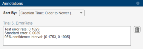
The function displays a summary of these statistics in the MATLAB Command Window.
Test error rate: 0.1829 Standard error: 0.0039 95% confidence interval: [0.1753, 0.1905]
To record observations about the results of your experiment, add an annotation:
- In the results table, right-click the ErrorRate cell of the best trial.
- Select Add Annotation.
- In the Annotations pane, enter your observations in the text box.
Close Experiment
In the Experiment Browser pane, right-click CIFARBayesianOptimizationProject and select Close Project. Experiment Manager closes the experiment and results contained in the project.
Setup Function
This function configures the training data, network architecture, and training options for the experiment. The input to this function is a structure with fields from the hyperparameter table. The function returns three outputs that you use to train a network for image classification problems.
function [augimdsTrain,layers,options] = BayesOptExperiment_setup(params)
Load Training Data
datadir = tempdir; downloadCIFARData(datadir);
[XTrain,YTrain,XTest,YTest] = loadCIFARData(datadir);
idx = randperm(numel(YTest),5000); XValidation = XTest(:,:,:,idx); YValidation = YTest(idx);
imageSize = [32 32 3];
pixelRange = [-4 4]; imageAugmenter = imageDataAugmenter( ... RandXReflection=true, ... RandXTranslation=pixelRange, ... RandYTranslation=pixelRange); augimdsTrain = augmentedImageDatastore(imageSize,XTrain,YTrain, ... DataAugmentation=imageAugmenter);
Define Network Architecture
numClasses = numel(unique(YTrain)); numF = round(16/sqrt(params.SectionDepth));
layers = [ imageInputLayer(imageSize)
convBlock(3,numF,params.SectionDepth)
maxPooling2dLayer(3,Stride=2,Padding="same")

convBlock(3,2*numF,params.SectionDepth)
maxPooling2dLayer(3,Stride=2,Padding="same")

convBlock(3,4*numF,params.SectionDepth)
averagePooling2dLayer(8)

fullyConnectedLayer(numClasses)
softmaxLayer
classificationLayer];
Specify Training Options
miniBatchSize = 256; validationFrequency = floor(numel(YTrain)/miniBatchSize);
options = trainingOptions("sgdm", ... InitialLearnRate=params.InitialLearnRate, ... Momentum=params.Momentum, ... MaxEpochs=60, ... LearnRateSchedule="piecewise", ... LearnRateDropPeriod=40, ... LearnRateDropFactor=0.1, ... MiniBatchSize=miniBatchSize, ... L2Regularization=params.L2Regularization, ... Shuffle="every-epoch", ... Verbose=false, ... ValidationData={XValidation,YValidation}, ... ValidationFrequency=validationFrequency);
Create Block of Convolutional Layers
This function creates a block of numConvLayers convolutional layers, each with a specified filterSize and numFilters filters, and each followed by a batch normalization layer and a ReLU layer.
function layers = convBlock(filterSize,numFilters,numConvLayers)
layers = [ convolution2dLayer(filterSize,numFilters,Padding="same") batchNormalizationLayer reluLayer]; layers = repmat(layers,numConvLayers,1);
end
Compute Error Rate
This metric function takes as input a structure that contains the fields trainedNetwork, trainingInfo, and parameters.
trainedNetworkis theSeriesNetworkobject orDAGNetworkobject returned by thetrainNetworkfunction.trainingInfois a structure containing the training information returned by thetrainNetworkfunction.parametersis a structure with fields from the hyperparameter table.
The function selects 5000 test images and labels, evaluates the trained network on the test set, calculates the predicted image labels, and calculates the error rate on the test data.
function metricOutput = ErrorRate(trialInfo)
datadir = tempdir;
[,,XTest,YTest] = loadCIFARData(datadir);
idx = randperm(numel(YTest),5000); XTest = XTest(:,:,:,idx); YTest = YTest(idx); YPredicted = classify(trialInfo.trainedNetwork,XTest);
metricOutput = 1 - mean(YPredicted == YTest); end
Summarize Test Statistics
This function computes the test error, standard error, and an approximate 95% confidence interval and displays a summary of these statistics in the MATLAB Command Window. The function also some test images together with their predicted classes and the probabilities of those classes.
function testSummary(net)
datadir = tempdir;
[,,XTest,YTest] = loadCIFARData(datadir);
[YPredicted,probs] = classify(net,XTest); testError = 1 - mean(YPredicted == YTest); NTest = numel(YTest); testErrorSE = sqrt(testError*(1-testError)/NTest); testError95CI = [testError - 1.96testErrorSE, testError + 1.96testErrorSE];
fprintf("\n\n\n"); fprintf("Test error rate: %.4f\n",testError); fprintf("Standard error: %.4f\n",testErrorSE); fprintf("95%% confidence interval: [%.4f, %.4f]\n",testError95CI(1),testError95CI(2)); fprintf("\n\n\n");
figure idx = randperm(numel(YTest),9); for i = 1:numel(idx) subplot(3,3,i) imshow(XTest(:,:,:,idx(i))); prob = num2str(100*max(probs(idx(i),:)),3); predClass = string(YPredicted(idx(i))); label = predClass+": "+prob+"%"; title(label) end end
See Also
Apps
Functions
- trainNetwork | trainingOptions | bayesopt (Statistics and Machine Learning Toolbox) | bestPoint (Statistics and Machine Learning Toolbox) | optimizableVariable (Statistics and Machine Learning Toolbox)
Related Topics
- Deep Learning Using Bayesian Optimization
- Evaluate Deep Learning Experiments by Using Metric Functions
- Use Bayesian Optimization in Custom Training Experiments
- Run Experiments in Parallel
- Offload Experiments as Batch Jobs to a Cluster
- Bayesian Optimization Algorithm (Statistics and Machine Learning Toolbox)