Evaluate Performance of Accelerated Deep Learning Function - MATLAB & Simulink (original) (raw)
This example shows how to evaluate the performance gains of using an accelerated function.
When using the dlfeval function in a custom training loop, the software traces each input dlarray object of the model loss function to determine the computation graph used for automatic differentiation. This tracing process can take some time and can spend time recomputing the same trace. By optimizing, caching, and reusing the traces, you can speed up gradient computation in deep learning functions. You can also optimize, cache, and reuse traces to accelerate other deep learning functions that do not require automatic differentiation, for example you can also accelerate model functions and functions used for prediction.
To speed up calls to deep learning functions, use the dlaccelerate function to create an AcceleratedFunction object that automatically optimizes, caches, and reuses the traces. You can use the dlaccelerate function to accelerate model functions and model loss functions directly, or to accelerate subfunctions used by these functions. The performance gains are most noticeable for deeper networks and training loops with many epochs and iterations.
The returned AcceleratedFunction object caches the traces of calls to the underlying function and reuses the cached result when the same input pattern reoccurs.
Try using dlaccelerate for function calls that:
- are long-running
- have
dlarrayobject, structures ofdlarrayobjects, ordlnetworkobjects as inputs - do not have side effects like writing to files or displaying output
This example compares training and prediction times when using and not using acceleration.
Load Training and Test Data
The digitTrain4DArrayData function loads the images, their digit labels, and their angles of rotation from the vertical. Create arrayDatastore objects for the images, labels, and angles, and then use the combine function to make a single datastore that contains all of the training data. Extract the class names and number of nondiscrete responses.
[imagesTrain,labelsTrain,anglesTrain] = digitTrain4DArrayData;
dsImagesTrain = arrayDatastore(imagesTrain,'IterationDimension',4); dsLabelsTrain = arrayDatastore(labelsTrain); dsAnglesTrain = arrayDatastore(anglesTrain);
dsTrain = combine(dsImagesTrain,dsLabelsTrain,dsAnglesTrain);
classNames = categories(labelsTrain); numClasses = numel(classNames); numResponses = size(anglesTrain,2); numObservations = numel(labelsTrain);
Create a datastore containing the test data given by the digitTest4DArrayData function using the same steps.
[imagesTest,labelsTest,anglesTest] = digitTest4DArrayData;
dsImagesTest = arrayDatastore(imagesTest,'IterationDimension',4); dsLabelsTest = arrayDatastore(labelsTest); dsAnglesTest = arrayDatastore(anglesTest);
dsTest = combine(dsImagesTest,dsLabelsTest,dsAnglesTest);
Define Deep Learning Model
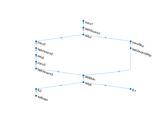
Define the following network that predicts both labels and angles of rotation.
- A convolution-batchnorm-ReLU block with 16 5-by-5 filters.
- A branch of two convolution-batchnorm blocks each with 32 3-by-3 filters with a ReLU operation between
- A skip connection with a convolution-batchnorm block with 32 1-by-1 convolutions.
- Combine both branches using addition followed by a ReLU operation
- For the regression output, a branch with a fully connected operation of size 1 (the number of responses).
- For classification output, a branch with a fully connected operation of size 10 (the number of classes) and a softmax operation.
Define and Initialize Model Parameters and State
Create a struct parametersBaseline containing the model parameters using the modelParameters function, listed at the end of the example. The modelParameters function creates structures parameters and state that contain the initialized model parameters and state, respectively.
The output uses the format parameters.OperationName.ParameterName where parameters is the structure, OperationName is the name of the operation (for example "conv1") and ParameterName is the name of the parameter (for example, "Weights").
[parametersBaseline,stateBaseline] = modelParameters(numClasses,numResponses);
Create a copy of the parameters and state for the baseline model to use for the accelerated model.
parametersAccelerated = parametersBaseline; stateAccelerated = stateBaseline;
Define Model Function
Create the function model, listed at the end of the example, that computes the outputs of the deep learning model described earlier.
The function model takes the model parameters parameters, the input data X, the flag doTraining which specifies whether to model should return outputs for training or prediction, and the network state state. The network outputs the predictions for the labels, the predictions for the angles, and the updated network state.
Define Model Loss Function
Create the function modelLoss, listed at the end of the example, that takes the model parameters, a mini-batch of input data X with corresponding targets T1 and T2 containing the labels and angles, respectively, and returns the loss, the updated network state, and the gradients of the loss with respect to the learnable parameters.
Specify Training Options
Specify the training options. Train for 20 epochs with a mini-batch size of 32. Displaying the plot can make training take longer to complete. Disable the plot by setting the plots variable to "none". To enable the plot, set this variable to "training-progress".
numEpochs = 20; miniBatchSize = 32; plots = "none";
Train Baseline Model
Use minibatchqueue to process and manage the mini-batches of images. For each mini-batch:
- Use the custom mini-batch preprocessing function
preprocessMiniBatch(defined at the end of this example) to one-hot encode the class labels. - Format the image data with the dimension labels
'SSCB'(spatial, spatial, channel, batch). By default, theminibatchqueueobject converts the data todlarrayobjects with underlying typesingle. Do not add a format to the class labels or angles. - Discard any partial mini-batches returned at the end of an epoch.
- Train on a GPU if one is available. By default, the
minibatchqueueobject converts each output to agpuArrayif a GPU is available. Using a GPU requires Parallel Computing Toolbox™ and a supported GPU device. For information on supported devices, see GPU Computing Requirements (Parallel Computing Toolbox).
mbq = minibatchqueue(dsTrain,... 'MiniBatchSize',miniBatchSize,... 'MiniBatchFcn',@preprocessMiniBatch,... 'MiniBatchFormat',{'SSCB','',''}, ... 'PartialMiniBatch','discard');
Initialize parameters for Adam.
trailingAvg = []; trailingAvgSq = [];
If required, initialize the training progress plot.
if plots == "training-progress" figure lineLossTrain = animatedline('Color',[0.85 0.325 0.098]); ylim([0 inf]) xlabel("Iteration") ylabel("Loss") grid on end
Train the model. For each epoch, shuffle the data and loop over mini-batches of data. For each mini-batch:
- Evaluate the model loss and gradients using
dlfevaland themodelLossfunction. - Update the network parameters using the
adamupdatefunction. - Update the training progress plot.
iteration = 0; start = tic;
% Loop over epochs. for epoch = 1:numEpochs
% Shuffle data.
shuffle(mbq)

% Loop over mini-batches
while hasdata(mbq)

    iteration = iteration + 1;

    [X,T1,T2] = next(mbq);

    % Evaluate the model loss, state, and gradients using dlfeval and the
    % model loss function.
    [loss,stateBaseline,gradients] = dlfeval(@modelLoss,parametersBaseline,X,T1,T2,stateBaseline);

    % Update the network parameters using the Adam optimizer.
    [parametersBaseline,trailingAvg,trailingAvgSq] = adamupdate(parametersBaseline,gradients, ...
        trailingAvg,trailingAvgSq,iteration);

    % Display the training progress.
    if plots == "training-progress"
        D = duration(0,0,toc(start),'Format','hh:mm:ss');
        loss = double(loss);
        addpoints(lineLossTrain,iteration,loss)
        title("Epoch: " + epoch + ", Elapsed: " + string(D))
        drawnow
    end
end
end elapsedBaseline = toc(start)
elapsedBaseline = 225.8675
Train Accelerated Model
Accelerate the model loss function using the dlaccelerate function.
accfun = dlaccelerate(@modelLoss);
Clear any previously cached traces of the accelerated function using the clearCache function.
Initialize parameters for Adam.
trailingAvg = []; trailingAvgSq = [];
If required, initialize the training progress plot.
if plots == "training-progress" figure lineLossTrain = animatedline('Color',[0.85 0.325 0.098]); ylim([0 inf]) xlabel("Iteration") ylabel("Loss") grid on end
Train the model using the accelerated model loss function in the call to the dlfeval function.
iteration = 0; start = tic;
% Loop over epochs. for epoch = 1:numEpochs
% Shuffle data.
shuffle(mbq)

% Loop over mini-batches
while hasdata(mbq)

    iteration = iteration + 1;

    [X,T1,T2] = next(mbq);

    % Evaluate the model loss, state, and gradients using dlfeval and the
    % accelerated function.
    [loss,stateAccelerated,gradients] = dlfeval(accfun, parametersAccelerated, X, T1, T2, stateAccelerated);

    % Update the network parameters using the Adam optimizer.
    [parametersAccelerated,trailingAvg,trailingAvgSq] = adamupdate(parametersAccelerated,gradients, ...
        trailingAvg,trailingAvgSq,iteration);

    % Display the training progress.
    if plots == "training-progress"
        D = duration(0,0,toc(start),'Format','hh:mm:ss');
        loss = double(loss);
        addpoints(lineLossTrain,iteration,loss)
        title("Epoch: " + epoch + ", Elapsed: " + string(D))
        drawnow
    end
end
end elapsedAccelerated = toc(start)
elapsedAccelerated = 151.9836
Check the efficiency of the accelerated function by inspecting the HitRate property. The HitRate property contains the percentage of function calls that reuse a cached trace.
Compare Training Times
Compare the training times in a bar chart.
figure bar(categorical(["Baseline" "Accelerated"]),[elapsedBaseline elapsedAccelerated]); ylabel("Time (seconds)") title("Training Time")
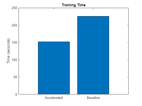
Calculate the speedup of acceleration.
speedup = elapsedBaseline / elapsedAccelerated
Time Baseline Predictions
Measure the time required to make predictions using the test data set.
After training, making predictions on new data does not require the labels. Create minibatchqueue object containing only the predictors of the test data:
- To ignore the labels for testing, set the number of outputs of the mini-batch queue to 1.
- Specify the same mini-batch size used for training.
- Preprocess the predictors using the
preprocessMiniBatchPredictorsfunction, listed at the end of the example. - For the single output of the datastore, specify the mini-batch format
'SSCB'(spatial, spatial, channel, batch).
numOutputs = 1; mbqTest = minibatchqueue(dsTest,numOutputs, ... 'MiniBatchSize',miniBatchSize, ... 'MiniBatchFcn',@preprocessMiniBatchPredictors, ... 'MiniBatchFormat','SSCB');
Loop over the mini-batches and classify the images using the modelPredictions function, listed at the end of the example and measure the elapsed time.
tic [labelsPred,anglesPred] = modelPredictions(@model,parametersBaseline,stateBaseline,mbqTest,classNames); elapsedPredictionBaseline = toc
elapsedPredictionBaseline = 5.3212
Time Accelerated Predictions
Because the model predictions function requires a mini-batch queue as input, the function does not support acceleration. To speed up prediction, accelerate the model function.
Accelerate the model function using the dlaccelerate function.
accfun2 = dlaccelerate(@model);
Clear any previously cached traces of the accelerated function using the clearCache function.
Reset the mini-batch queue.
Loop over the mini-batches and classify the images using the modelPredictions function, listed at the end of the example and measure the elapsed time.
tic [labelsPred,anglesPred] = modelPredictions(accfun2,parametersBaseline,stateBaseline,mbqTest,classNames); elapsedPredictionAccelerated = toc
elapsedPredictionAccelerated = 4.2596
Check the efficiency of the accelerated function by inspecting the HitRate property. The HitRate property contains the percentage of function calls that reuse a cached trace.
Compare Prediction Times
Compare the prediction times in a bar chart.
figure bar(categorical(["Baseline" "Accelerated"]),[elapsedPredictionBaseline elapsedPredictionAccelerated]); ylabel("Time (seconds)") title("Prediction Time")
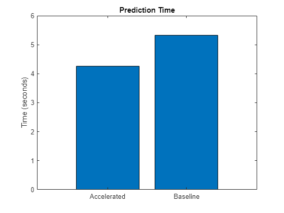
Calculate the speedup of acceleration.
speedup = elapsedPredictionBaseline / elapsedPredictionAccelerated
Model Parameters Function
The modelParameters function creates structures parameters and state that contain the initialized model parameters and state, respectively for the model described in the Define Deep Learning Model section. The function takes as input the number of classes and the number of responses and initializes the learnable parameters. The function:
- initializes the layer weights using the
initializeGlorotfunction - initializes the layer biases using the
initializeZerosfunction - initializes the batch normalization offset and scale parameters with the
initializeZerosfunction - initializes the batch normalization scale parameters with the
initializeOnesfunction - initializes the batch normalization state trained mean with the
initializeZerosfunction - initializes the batch normalization state trained variance with the
initializeOnesexample function
The initialization example functions are attached to this example as supporting files. To access these files, open the example as a live script. To learn more about initializing learnable parameters for deep learning models, see Initialize Learnable Parameters for Model Function.
The output uses the format parameters.OperationName.ParameterName where parameters is the structure, OperationName is the name of the operation (for example "conv1") and ParameterName is the name of the parameter (for example, "Weights").
function [parameters,state] = modelParameters(numClasses,numResponses)
% First convolutional layer. filterSize = [5 5]; numChannels = 1; numFilters = 16;
sz = [filterSize numChannels numFilters]; numOut = prod(filterSize) * numFilters; numIn = prod(filterSize) * numFilters;
parameters.conv1.Weights = initializeGlorot(sz,numOut,numIn); parameters.conv1.Bias = initializeZeros([numFilters 1]);
% First batch normalization layer. parameters.batchnorm1.Offset = initializeZeros([numFilters 1]); parameters.batchnorm1.Scale = initializeOnes([numFilters 1]); state.batchnorm1.TrainedMean = initializeZeros([numFilters 1]); state.batchnorm1.TrainedVariance = initializeOnes([numFilters 1]);
% Second convolutional layer. filterSize = [3 3]; numChannels = 16; numFilters = 32;
sz = [filterSize numChannels numFilters]; numOut = prod(filterSize) * numFilters; numIn = prod(filterSize) * numFilters;
parameters.conv2.Weights = initializeGlorot(sz,numOut,numIn); parameters.conv2.Bias = initializeZeros([numFilters 1]);
% Second batch normalization layer. parameters.batchnorm2.Offset = initializeZeros([numFilters 1]); parameters.batchnorm2.Scale = initializeOnes([numFilters 1]); state.batchnorm2.TrainedMean = initializeZeros([numFilters 1]); state.batchnorm2.TrainedVariance = initializeOnes([numFilters 1]);
% Third convolutional layer. filterSize = [3 3]; numChannels = 32; numFilters = 32;
sz = [filterSize numChannels numFilters]; numOut = prod(filterSize) * numFilters; numIn = prod(filterSize) * numFilters;
parameters.conv3.Weights = initializeGlorot(sz,numOut,numIn); parameters.conv3.Bias = initializeZeros([numFilters 1]);
% Third batch normalization layer. parameters.batchnorm3.Offset = initializeZeros([numFilters 1]); parameters.batchnorm3.Scale = initializeOnes([numFilters 1]); state.batchnorm3.TrainedMean = initializeZeros([numFilters 1]); state.batchnorm3.TrainedVariance = initializeOnes([numFilters 1]);
% Convolutional layer in the skip connection. filterSize = [1 1]; numChannels = 16; numFilters = 32;
sz = [filterSize numChannels numFilters]; numOut = prod(filterSize) * numFilters; numIn = prod(filterSize) * numFilters;
parameters.convSkip.Weights = initializeGlorot(sz,numOut,numIn); parameters.convSkip.Bias = initializeZeros([numFilters 1]);
% Batch normalization layer in the skip connection. parameters.batchnormSkip.Offset = initializeZeros([numFilters 1]); parameters.batchnormSkip.Scale = initializeOnes([numFilters 1]);
state.batchnormSkip.TrainedMean = initializeZeros([numFilters 1]); state.batchnormSkip.TrainedVariance = initializeOnes([numFilters 1]);
% Fully connected layer corresponding to the classification output. sz = [numClasses 6272]; numOut = numClasses; numIn = 6272; parameters.fc1.Weights = initializeGlorot(sz,numOut,numIn); parameters.fc1.Bias = initializeZeros([numClasses 1]);
% Fully connected layer corresponding to the regression output. sz = [numResponses 6272]; numOut = numResponses; numIn = 6272; parameters.fc2.Weights = initializeGlorot(sz,numOut,numIn); parameters.fc2.Bias = initializeZeros([numResponses 1]);
end
Model Function
The function model takes the model parameters parameters, the input data X, the flag doTraining which specifies whether to model should return outputs for training or prediction, and the network state state. The network outputs the predictions for the labels, the predictions for the angles, and the updated network state.
function [Y1,Y2,state] = model(parameters,X,doTraining,state)
% Convolution weights = parameters.conv1.Weights; bias = parameters.conv1.Bias; Y = dlconv(X,weights,bias,'Padding','same');
% Batch normalization, ReLU offset = parameters.batchnorm1.Offset; scale = parameters.batchnorm1.Scale; trainedMean = state.batchnorm1.TrainedMean; trainedVariance = state.batchnorm1.TrainedVariance;
if doTraining [Y,trainedMean,trainedVariance] = batchnorm(Y,offset,scale,trainedMean,trainedVariance);
% Update state
state.batchnorm1.TrainedMean = trainedMean;
state.batchnorm1.TrainedVariance = trainedVariance;
else Y = batchnorm(Y,offset,scale,trainedMean,trainedVariance); end
Y = relu(Y);
% Convolution, batch normalization (Skip connection) weights = parameters.convSkip.Weights; bias = parameters.convSkip.Bias; YSkip = dlconv(Y,weights,bias,'Stride',2);
offset = parameters.batchnormSkip.Offset; scale = parameters.batchnormSkip.Scale; trainedMean = state.batchnormSkip.TrainedMean; trainedVariance = state.batchnormSkip.TrainedVariance;
if doTraining [YSkip,trainedMean,trainedVariance] = batchnorm(YSkip,offset,scale,trainedMean,trainedVariance);
% Update state
state.batchnormSkip.TrainedMean = trainedMean;
state.batchnormSkip.TrainedVariance = trainedVariance;
else YSkip = batchnorm(YSkip,offset,scale,trainedMean,trainedVariance); end
% Convolution weights = parameters.conv2.Weights; bias = parameters.conv2.Bias; Y = dlconv(Y,weights,bias,'Padding','same','Stride',2);
% Batch normalization, ReLU offset = parameters.batchnorm2.Offset; scale = parameters.batchnorm2.Scale; trainedMean = state.batchnorm2.TrainedMean; trainedVariance = state.batchnorm2.TrainedVariance;
if doTraining [Y,trainedMean,trainedVariance] = batchnorm(Y,offset,scale,trainedMean,trainedVariance);
% Update state
state.batchnorm2.TrainedMean = trainedMean;
state.batchnorm2.TrainedVariance = trainedVariance;
else Y = batchnorm(Y,offset,scale,trainedMean,trainedVariance); end
Y = relu(Y);
% Convolution weights = parameters.conv3.Weights; bias = parameters.conv3.Bias; Y = dlconv(Y,weights,bias,'Padding','same');
% Batch normalization offset = parameters.batchnorm3.Offset; scale = parameters.batchnorm3.Scale; trainedMean = state.batchnorm3.TrainedMean; trainedVariance = state.batchnorm3.TrainedVariance;
if doTraining [Y,trainedMean,trainedVariance] = batchnorm(Y,offset,scale,trainedMean,trainedVariance);
% Update state
state.batchnorm3.TrainedMean = trainedMean;
state.batchnorm3.TrainedVariance = trainedVariance;
else Y = batchnorm(Y,offset,scale,trainedMean,trainedVariance); end
% Addition, ReLU Y = YSkip + Y; Y = relu(Y);
% Fully connect, softmax (labels) weights = parameters.fc1.Weights; bias = parameters.fc1.Bias; Y1 = fullyconnect(Y,weights,bias); Y1 = softmax(Y1);
% Fully connect (angles) weights = parameters.fc2.Weights; bias = parameters.fc2.Bias; Y2 = fullyconnect(Y,weights,bias);
end
Model Loss Function
The modelLoss function, takes the model parameters, a mini-batch of input data X with corresponding targets T1 and T2 containing the labels and angles, respectively, and returns the loss, the updated network state, and the gradients of the loss with respect to the learnable parameters.
function [loss,state,gradients] = modelLoss(parameters,X,T1,T2,state)
doTraining = true; [Y1,Y2,state] = model(parameters,X,doTraining,state);
lossLabels = crossentropy(Y1,T1); lossAngles = mse(Y2,T2);
loss = lossLabels + 0.1*lossAngles; gradients = dlgradient(loss,parameters);
end
Model Predictions Function
The modelPredictions function takes the model parameters, state, a minibatchqueue of input data mbq, and the network classes, and computes the model predictions by iterating over all data in the minibatchqueue object. The function uses the onehotdecode function to find the predicted class with the highest score.
function [predictions1, predictions2] = modelPredictions(modelFcn,parameters,state,mbq,classes)
doTraining = false; predictions1 = []; predictions2 = [];
while hasdata(mbq)
XTest = next(mbq);

[YPred1,YPred2] = modelFcn(parameters,XTest,doTraining,state);

YPred1 = onehotdecode(YPred1,classes,1)';
YPred2 = extractdata(YPred2)';

predictions1 = [predictions1; YPred1];
predictions2 = [predictions2; YPred2];
end
end
Mini-Batch Preprocessing Function
The preprocessMiniBatch function preprocesses the data using the following steps:
- Extract the image data from the incoming cell array and concatenate into a numeric array. Concatenating the image data over the fourth dimension adds a third dimension to each image, to be used as a singleton channel dimension.
- Extract the label and angle data from the incoming cell arrays and concatenate along the second dimension into a categorical array and a numeric array, respectively.
- One-hot encode the categorical labels into numeric arrays. Encoding into the first dimension produces an encoded array that matches the shape of the network output.
function [X,Y,angle] = preprocessMiniBatch(XCell,YCell,angleCell)
% Preprocess predictors. X = preprocessMiniBatchPredictors(XCell);
% Extract label data from cell and concatenate Y = cat(2,YCell{:});
% Extract angle data from cell and concatenate angle = cat(2,angleCell{:});
% One-hot encode labels Y = onehotencode(Y,1);
end
Mini-Batch Predictors Preprocessing Function
The preprocessMiniBatchPredictors function preprocesses a mini-batch of predictors by extracting the image data from the input cell array and concatenate into a numeric array. For grayscale input, concatenating over the fourth dimension adds a third dimension to each image, to use as a singleton channel dimension.
function X = preprocessMiniBatchPredictors(XCell)
% Concatenate. X = cat(4,XCell{1:end});
end
See Also
dlaccelerate | AcceleratedFunction | clearCache | dlarray | dlgradient | dlfeval