Train Network in Parallel with Custom Training Loop - MATLAB & Simulink (original) (raw)

Main Content

This example shows how to set up a custom training loop to train a network in parallel.

Training deep neural networks is computationally expensive and can take many hours of computing time. To speed up training, particularly when you have multiple GPUs, you can train a network in parallel.

In this example, parallel workers train on portions of the overall mini-batch. If you have a GPU, then training happens on the GPU. During training, a DataQueue object sends training progress information back to the MATLAB client.

Load Data Set

Download and extract the Flowers data set [1]. The Flowers data set contains 3670 images of flowers belonging to five classes (daisy, dandelion, roses, sunflowers, and tulips).

url = "http://download.tensorflow.org/example_images/flower_photos.tgz"; downloadFolder = tempdir; filename = fullfile(downloadFolder,"flower_dataset.tgz");

dataFolder = fullfile(downloadFolder,"flower_photos"); if ~exist(dataFolder,"dir") fprintf("Downloading Flowers data set (218 MB)... ") websave(filename,url); untar(filename,downloadFolder) fprintf("Done.\n") end

Downloading Flowers data set (218 MB)...

Create an image datastore for the data set. Randomly split the datastore into training and test datastores.

imds = imageDatastore(dataFolder, ... IncludeSubfolders=true, ... LabelSource="foldernames");

[imdsTrain,imdsTest] = splitEachLabel(imds,0.9,"randomized");

To resize the training images, create an augmentedImageDatastore. Shuffle the data with the shuffle function.

inputSize = [100 100 3]; augimdsTrain = augmentedImageDatastore(inputSize(1:2),imdsTrain); augimdsTrain = shuffle(augimdsTrain);

Determine the different classes in the training data set.

classes = categories(imdsTrain.Labels)

classes = 5×1 cell {'daisy' } {'dandelion' } {'roses' } {'sunflowers'} {'tulips' }

numClasses = numel(classes)

Define Network

Create a 2-D residual network. This network architecture includes batch normalization layers, which track the mean and variance statistics of the data set. When training in parallel, combine the statistics from all of the workers at the end of each iteration step, to ensure the network state reflects the whole mini-batch. Otherwise, the network state can diverge across the workers.

net = resnetNetwork(inputSize,numClasses)

net = dlnetwork with properties:

     Layers: [176×1 nnet.cnn.layer.Layer]
Connections: [191×2 table]
 Learnables: [214×3 table]
      State: [106×3 table]
 InputNames: {'input'}
OutputNames: {'softmax'}
Initialized: 1

View summary with summary.

If you instead use a recurrent neural network (RNN), for example, a network containing LSTM or GRU layers, the recurrent layers have state properties that change during training. You must therefore take care to manage these states when you train a network in parallel using a custom training loop. To train an RNN statelessly, i.e. without maintaining the state of the recurrent layers between training iterations, call resetState at the end of each training iteration. You do not need to edit the code for aggregating batch normalization statistics across the workers.

Set Up Parallel Environment

Determine if GPUs are available for MATLAB to use with the canUseGPU function. Using a GPU requires Parallel Computing Toolbox™ and a supported GPU device. For information on supported devices, see GPU Computing Requirements (Parallel Computing Toolbox).

If there are GPUs available, then train on the GPUs. Create a parallel pool with as many workers as GPUs.
If there are no GPUs available, then train on the CPUs. Create a parallel pool with the default number of workers.

if canUseGPU executionEnvironment = "gpu"; numberOfGPUs = gpuDeviceCount("available"); gpuDeviceTable pool = parpool(numberOfGPUs); else executionEnvironment = "cpu"; pool = parpool; end

ans=4×5 table Index Name ComputeCapability DeviceAvailable DeviceSelected _____ _________________ _________________ _______________ ______________

  1      "NVIDIA TITAN Xp"          "6.1"               true              true      
  2      "NVIDIA TITAN Xp"          "6.1"               true              false     
  3      "NVIDIA TITAN Xp"          "6.1"               true              false     
  4      "NVIDIA TITAN Xp"          "6.1"               true              false

Starting parallel pool (parpool) using the 'Processes' profile ...

Get the number of workers in the parallel pool.

numWorkers = pool.NumWorkers;

Train Model

Specify the training options.

numEpochs = 100; miniBatchSize = 128; velocity = [];

For GPU training, a recommended practice is to scale up the mini-batch size linearly with the number of GPUs, in order to keep the workload on each GPU constant. For more related advice, see Deep Learning with MATLAB on Multiple GPUs.

if executionEnvironment == "gpu" miniBatchSize = miniBatchSize .* numWorkers end

Calculate the mini-batch size for each worker by dividing the overall mini-batch size evenly among the workers. Distribute the remainder across the first workers.

workerMiniBatchSize = floor(miniBatchSize ./ repmat(numWorkers,1,numWorkers)); remainder = miniBatchSize - sum(workerMiniBatchSize); workerMiniBatchSize = workerMiniBatchSize + [ones(1,remainder) zeros(1,numWorkers-remainder)]

workerMiniBatchSize = 128

This network contains batch normalization layers that keep track of the mean and variance of the data the network is trained on. Since each worker processes a portion of each mini-batch during each iteration, the mean and variance must be aggregated across all the workers. Find the names of all of the batch normalization layers in the network.

layers = net.Layers; batchNormLayersNames = string.empty;

for idx = 1:numel(layers) currentLayer = layers(idx); if isa(currentLayer,"nnet.cnn.layer.BatchNormalizationLayer") batchNormLayersNames(end+1) = currentLayer.Name; end end

Find the indices of the mean and variance state parameters of the batch normalization layers in the network state property.

state = net.State; isBatchNormalizationStateMean = ismember(state.Layer,batchNormLayersNames) & state.Parameter == "TrainedMean"; isBatchNormalizationStateVariance = ismember(state.Layer,batchNormLayersNames) & state.Parameter == "TrainedVariance";

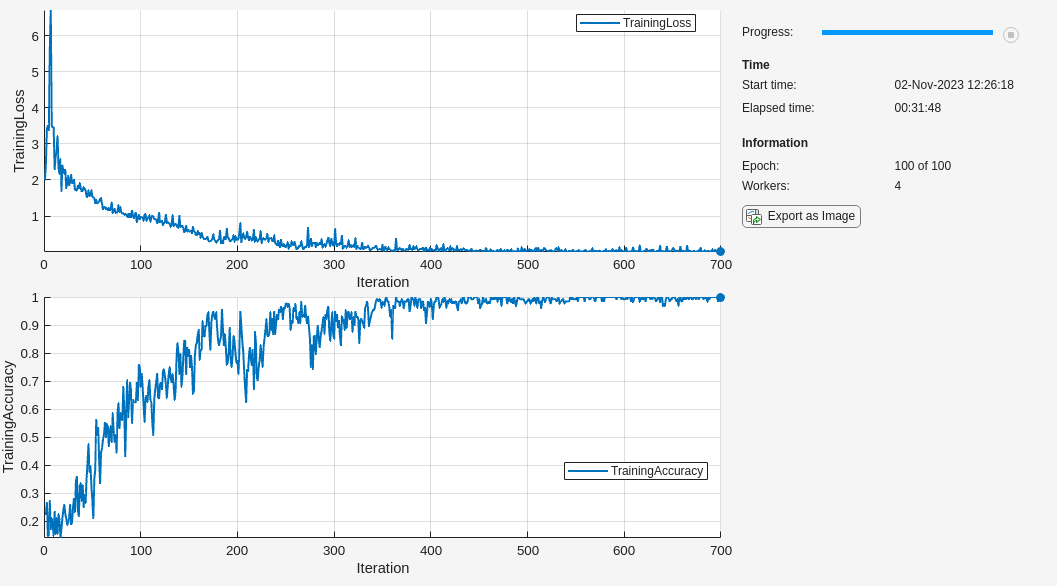
Initialize the TrainingProgressMonitor object. Because the timer starts when you create the monitor object, make sure that you create the object close to the training loop.

monitor = trainingProgressMonitor( ... Metrics=["TrainingLoss" "TrainingAccuracy"], ... Info=["Epoch" "Workers"], ... XLabel="Iteration");

Create a Dataqueue object on the workers to send a flag to stop training when the Stop button is clicked.

spmd stopTrainingEventQueue = parallel.pool.DataQueue; end stopTrainingQueue = stopTrainingEventQueue{1};

To send data back from the workers during training, create a DataQueue object. Use afterEach to set up a function, displayTrainingProgress, to call each time a worker sends data. displayTrainingProgress is a supporting function, defined at the end of this example, that displays updates the TrainingProgressMonitor object to show the training progress information that comes from the workers and sends a flag to the workers if the Stop button has been clicked.

dataQueue = parallel.pool.DataQueue; displayFcn = @(x) displayTrainingProgress(x,numEpochs,numWorkers,monitor,stopTrainingQueue); afterEach(dataQueue,displayFcn)

Train the model using a custom parallel training loop, as detailed in the following steps. To execute the code simultaneously on all the workers, use an spmd block. Within the spmd block, spmdIndex gives the index of the worker currently executing the code.

Before training, partition the datastore for each worker by using the partition function. Use the partitioned datastore to create a minibatchqueue on each worker. For each mini-batch:

Use the custom mini-batch preprocessing function preprocessMiniBatch (defined at the end of this example) to normalize the data, convert the target classes to one-hot encoded variables, and determine the number of observations in the mini-batch.
Format the image data with the dimension labels "SSCB" (spatial, spatial, channel, batch). By default, the minibatchqueue object converts the data to dlarray objects with underlying type single. Do not add a format to the target classes or the number of observations.
Train on a GPU if one is available. By default, the minibatchqueue object converts each output to a gpuArray if a GPU is available.
Accelerate the model loss function using the dlaccelerate function. For more information about deep learning function acceleration, see Deep Learning Function Acceleration for Custom Training Loops.

For each epoch, shuffle the datastore with the shuffle function. For each iteration in the epoch:

Ensure that all workers have data available before beginning processing it in parallel. The continueEpoch function is a supporting function defined at the end of this example and ensures that all workers have data available by concatenating the result of the hasdata function across the workers using the spmdCat function.
Check whether the Stop button has been clicked. The continueEpoch function checks this by monitoring the length of the stopTrainingEveneQueue.
Read a mini-batch from the minibatchqueue by using the next function.
Compute the loss and the gradients of the network on each worker by calling dlfeval on the modelLoss function. The dlfeval function evaluates the helper function modelLoss with automatic differentiation enabled, so modelLoss can compute the gradients with respect to the loss in an automatic way. modelLoss is defined at the end of the example and returns the loss and gradients given a network, mini-batch of data, and targets.
To obtain the overall loss, aggregate the losses on all workers. This example uses cross-entropy for the loss function, and the aggregated loss is the sum of all losses. Before aggregating, normalize each loss by multiplying by the proportion of the overall mini-batch that the worker is working on. Use spmdPlus to add all losses together and replicate the results across workers.
To aggregate and update the gradients of all workers, use the aggregateAllGradients function. aggregateAllGradients is a supporting function defined at the end of this example. This function uses spmdPlus to add together and replicate gradients across workers, following normalization according to the proportion of the overall mini-batch that each worker is working on.
Aggregate the state of the network on all workers using the aggregateState function. aggregateState is a supporting function defined at the end of this example. The batch normalization layers in the network track the mean and variance of the data. Since the complete mini-batch is spread across multiple workers, aggregate the network state after each iteration to compute the mean and variance of the whole mini-batch.
After computing the final gradients, update the network learnable parameters with the sgdmupdate function.
Send training progress information back to the client using the send function with the Dataqueue object. You only need to use one worker to send back data because all of the workers have the same loss information. To ensure that data is on the CPU and a client machine without a GPU can access it, use gather on the dlarray before sending it to the client.

spmd % Partition the datastore. workerImds = partition(augimdsTrain,numWorkers,spmdIndex);

% Create minibatchqueue using partitioned datastore on each worker.
workerMbq = minibatchqueue(workerImds,3,...
    MiniBatchSize=workerMiniBatchSize(spmdIndex),...
    MiniBatchFcn=@preprocessMiniBatch,...
    MiniBatchFormat=["SSCB" "" ""]);

% Use dlaccelerate on the modelLoss
accModelLoss = dlaccelerate(@modelLoss);

workerVelocity = velocity;
epoch = 0;
iteration = 0;

while epoch < numEpochs
    epoch = epoch + 1;
    shuffle(workerMbq);

    % Loop over mini-batches.
    while continueEpoch(workerMbq,stopTrainingEventQueue)
        iteration = iteration + 1;

        % Read a mini-batch of data.
        [workerX,workerT,workerNumObservations] = next(workerMbq);

        % Evaluate the model loss and gradients on the worker.
        [workerLoss,workerGradients,workerState] = dlfeval(accModelLoss,net,workerX,workerT);

        % Aggregate the losses on all workers.
        workerNormalizationFactor = workerMiniBatchSize(spmdIndex)./miniBatchSize;
        loss = spmdPlus(workerNormalizationFactor*extractdata(workerLoss));

        % Aggregate the network state on all workers.
        net.State = aggregateState(workerState,workerNormalizationFactor,...
            isBatchNormalizationStateMean,isBatchNormalizationStateVariance);

        % Aggregate the gradients on all workers.
        workerGradients.Value = aggregateAllGradients(workerGradients.Value,workerNormalizationFactor);
       
        % Update the network parameters using the SGDM optimizer.
        [net,workerVelocity] = sgdmupdate(net,workerGradients,workerVelocity);

        % Calculate the training accuracy and send training progress information to the client.
        if spmdIndex == 1
            scores = predict(net,workerX);
            labels = scores2label(workerT,classes);
            Y = scores2label(scores,classes);
            accuracy = mean(Y==labels);

            data = [epoch loss accuracy iteration];
            send(dataQueue,gather(data));
        end
    end

end

end

Test Model

After the training is complete, all workers have the same complete trained network. Retrieve any of them.

After you train the network, test its accuracy.

Classify the test images. To make predictions with multiple observations, use the minibatchpredict function. To convert the prediction scores to labels, use the scores2label function. The minibatchpredict function automatically uses a GPU if one is available. Otherwise, the function uses the CPU.

labels = imdsTest.Labels; imdsTestResized = transform(imdsTest,@(X) {imresize(X,inputSize(1:2))}); X = readall(imdsTestResized); X = cat(4,X{:}); X = single(X) ./ 255;

scores = minibatchpredict(netFinal,X); Y = scores2label(scores,classes);

Calculate the accuracy of the network.

accuracy = mean(Y==labels)

Mini Batch Preprocessing Function

The preprocessMiniBatch function preprocesses a mini-batch of predictors and target classes using the following steps:

Determine the number of observations in the mini-batch
Preprocess the images using the preprocessMiniBatchPredictors function.
Extract the target class data from the incoming cell array and concatenate into a categorical array along the second dimension.
One-hot encode the categorical labels into numeric arrays. Encoding into the first dimension produces an encoded array that matches the shape of the network output.

function [X,Y,numObs] = preprocessMiniBatch(XCell,YCell)

numObs = numel(YCell);

% Preprocess predictors. X = preprocessMiniBatchPredictors(XCell);

% Extract class data from cell and concatenate. Y = cat(2,YCell{1:end});

% One-hot encode classes. Y = onehotencode(Y,1);

end

Mini-Batch Predictors Preprocessing Function

The preprocessMiniBatchPredictors function preprocesses a mini-batch of predictors by extracting the image data from the input cell array and concatenate into a numeric array. The images are then normalized.

function X = preprocessMiniBatchPredictors(XCell)

X = cat(4,XCell{:});

X = single(X) ./ 255;

end

Model Loss Function

The modelLoss function computes the gradients of the loss with respect to the learnable parameters of the network. This function computes the network outputs for a mini-batch X with forward and calculates the loss, given the targets T, using cross entropy. When you call this function with dlfeval, automatic differentiation is enabled, and dlgradient can compute the gradients of the loss with respect to the learnables automatically.

function [loss,gradients,state] = modelLoss(net,X,T)

[Y,state] = forward(net,X);

loss = crossentropy(Y,T); gradients = dlgradient(loss,net.Learnables);

end

Display Training Progress Function

The displayTrainingProgress function displays training progress information that comes from the workers and checks whether the Stop button has been clicked. If the Stop button has been clicked, a flag is sent to the workers to indicate that training should stop. The DataQueue in this example calls this function every time a worker sends data.

function displayTrainingProgress(data,numEpochs,numWorkers,monitor,stopTrainingQueue)

% Extract training information from array. epoch = data(1); loss = data(2); accuracy = data(3); iteration = data(4);

% Update training progress monitor. recordMetrics(monitor,iteration,TrainingLoss=loss,TrainingAccuracy=accuracy); updateInfo(monitor,Epoch=epoch + " of " + numEpochs, Workers= numWorkers); monitor.Progress = 100 * epoch/numEpochs;

% Send flag if the Stop button is clicked. if monitor.Stop send(stopTrainingQueue,true); end

end

Aggregate Gradients Function

The aggregateAllGradients function aggregates the gradients on all workers by adding them together. spmdPlus adds together and replicates all the gradients on the workers. Before adding them together, normalize them by multiplying them by a factor that represents the proportion of the overall mini-batch that the worker is working on. To retrieve the contents of a dlarray, use extractdata.

function gradients = aggregateAllGradients(gradients,normalizationFactor)

% Inspect array of gradients and create cell array for storing aggregated % data. numArrays = numel(gradients); aggregationData = cell(numArrays); arraySizes = cell(numArrays,1); numElements = zeros(numArrays,1);

% Extract the data from all the arrays for idxArray = 1:numArrays data = gradients{idxArray}; gradients{idxArray} = [];

% Extract data from dlarray.
data = extractdata(data);

% Save the size of the array.
arraySizes{idxArray} = size(data);
numElements(idxArray) = numel(data);

% Flatten the array to prepare for concatenation.
aggregationData{idxArray} = data(:);

end

% Concatenate all arrays. aggregationData = cat(1,aggregationData{:});

% Aggregate the data from the workers. aggregationData = spmdPlus(normalizationFactor.*aggregationData);

% Reconstruct the gradient arrays. i = 1; for idxArray = 1:numArrays n = numElements(idxArray); if n > 0 % Reshape the flattened data to the original size. data = reshape(aggregationData(i:(i+n-1)),arraySizes{idxArray}); % Reinsert the aggregated data as a dlarray. gradients{idxArray} = dlarray(data); i = i + n; end end end

Aggregate State Function

The aggregateState function aggregates the network state on all workers. The network state contains the trained batch normalization statistics of the data set. Since each worker only sees a portion of the mini-batch, aggregate the network state so that the statistics are representative of the statistics across all the data. For each mini-batch, the combined mean is calculated as a weighted average of the mean across the workers for each iteration. The combined variance is calculated according to the following formula:

sc2=1M∑j=1Nmj[sj2+(x‾j-x‾c)2]

where Nis the total number of workers, Mis the total number of observations in a mini-batch, mj is the number of observations processed on the jth worker, x‾j and sj2 are the mean and variance statistics calculated on that worker, and x‾c is the combined mean across all workers.

function state = aggregateState(state,normalizationFactor,... isBatchNormalizationStateMean,isBatchNormalizationStateVariance)

stateMeans = state.Value(isBatchNormalizationStateMean); stateVariances = state.Value(isBatchNormalizationStateVariance);

for j = 1:numel(stateMeans) meanVal = stateMeans{j}; varVal = stateVariances{j};

% Calculate combined mean.
combinedMean = spmdPlus(normalizationFactor*meanVal);

% Calculate combined variance terms to sum.
varTerm = normalizationFactor.*(varVal + (meanVal - combinedMean).^2);

% Update state.
stateMeans{j} = combinedMean;
stateVariances{j} = spmdPlus(varTerm);

end

state.Value(isBatchNormalizationStateMean) = stateMeans; state.Value(isBatchNormalizationStateVariance) = stateVariances;

end

Continue Epoch Function

The continueEpoch function checks whether the mini-batch queue on each worker has data remaining and checks whether the Stop button has been pressed.

function tf = continueEpoch(workerMbq,stopTrainingEventQueue)

% Create a struct that will be concatenated across the workers. info.HasData = hasdata(workerMbq); info.StopRequested = stopTrainingEventQueue.QueueLength > 0;

% Use spmdCat to aggregate the info from all the workers. info = spmdCat(info);

% Continue training if all the workers have data, and if we were not asked to stop. stopRequest = any([info.StopRequested]); tf = ~stopRequest && all([info.HasData]);

end

References

The TensorFlow Team. Flowers http://download.tensorflow.org/example_images/flower_photos.tgz