dsp.FFT - Discrete Fourier transform - MATLAB (original) (raw)

Discrete Fourier transform

Description

The dsp.FFT System object™ computes the discrete Fourier transform (DFT) of an input using fast Fourier transform (FFT). The object uses one or more of the following fast Fourier transform (FFT) algorithms depending on the complexity of the input and whether the output is in linear or bit-reversed order:

Double-signal algorithm
Half-length algorithm
Radix-2 decimation-in-time (DIT) algorithm
Radix-2 decimation-in-frequency (DIF) algorithm
An algorithm chosen from FFTW [1] , [2]

The dsp.FFT object and the fft function both compute the discrete Fourier transform (DFT) using fast Fourier transform (FFT). However, the object can process large streams of real-time data and handle system states automatically. The function performs one-time computations on data that is readily available and cannot handle system states. For a comparison between the two, see System Objects vs MATLAB Functions.

To compute the DFT of an input:

Create the dsp.FFT object and set its properties.
Call the object with arguments, as if it were a function.

To learn more about how System objects work, see What Are System Objects?

Creation

Syntax

Description

`ft` = dsp.FFT returns aFFT object that computes the discrete Fourier transform (DFT) of a real or complex_N_-D array input along the first dimension using fast Fourier transform (FFT).

`ft` = dsp.FFT(`Name=Value`)sets properties using one or more name-value arguments. For example, to specify an FFT length of 128, set FFTLength to 128.

example

Properties

expand all

Unless otherwise indicated, properties are nontunable, which means you cannot change their values after calling the object. Objects lock when you call them, and therelease function unlocks them.

If a property is tunable, you can change its value at any time.

For more information on changing property values, seeSystem Design in MATLAB Using System Objects.

Specify the implementation used for the FFT as one of"Auto", "Radix-2", or"FFTW". When you set this property to"Radix-2", the FFT length must be a power of two.

Designate order of output channel elements relative to order of input elements. Set this property to true to output the frequency indices in bit-reversed order. The default isfalse, which corresponds to a linear ordering of frequency indices.

Set this property to true if the output of the FFT should be divided by the FFT length. This option is useful when you want the output of the FFT to stay in the same amplitude range as its input. This is particularly useful when working with fixed-point data types.

The default value of this property is false with no scaling.

Specify how to determine the FFT length as"Auto" or "Property". When you set this property to "Auto", the FFT length equals the number of rows of the input signal.

FFT length, specified as an integer greater than or equal to 2.

This property must be a power of two if any of these conditions apply:

The input is a fixed-point data type.
The BitReversedOutput property istrue.
The FFTImplementation property is"Radix-2".

Dependencies

This property applies when you set theFFTLengthSource property to"Property".

Wrap input data when FFT length is shorter than input length. If this property is set to true, modulo-length data wrapping occurs before the FFT operation, given FFT length is shorter than the input length. If this property is set to false, truncation of the input data to the FFT length occurs before the FFT operation.

Fixed-Point Properties

Specify the rounding method.

Specify the overflow action as "Wrap" or"Saturate".

Specify the sine table data type as "Same word length as input" or "Custom".

Specify the sine table fixed-point type as an unscalednumerictype (Fixed-Point Designer) object with a Signedness of"Auto".

Dependencies

This property applies when you set theSineTableDataType property to"Custom".

Specify the product data type as "Full precision", "Same as input", or"Custom".

Specify the product fixed-point type as a scaled numerictype (Fixed-Point Designer) object with a Signedness of"Auto".

Dependencies

This property applies when you set theProductDataType property to"Custom".

Specify the accumulator data type as "Full precision", "Same as input","Same as product", or"Custom".

Specify the accumulator fixed-point type as a scaled numerictype (Fixed-Point Designer) object with a Signedness of"Auto".

Dependencies

This property applies when you set theAccumulatorDataType property to"Custom".

Specify the output data type as one of "Full precision", "Same as input","Custom".

Specify the output fixed-point type as a scaled numerictype (Fixed-Point Designer) object with a Signedness of"Auto".

Dependencies

This property applies when you set the OutputDataType property to"Custom".

Usage

Syntax

Description

[y](#d126e275512) = ft([x](#d126e275424)) computes the DFT, y, of the inputx along the first dimension ofx.

example

Input Arguments

expand all

Time-domain input signal, specified as a vector, matrix, or_N_-D array.

When the FFTLengthSource property is set to "Auto", the length ofx along the first dimension must be a positive integer power of two. This length is also the FFT length. When the FFTLengthSource property is "Property", the value you specify in FFTLength property must be a positive integer power of two.

Variable-size input signals are only supported when theFFTLengthSource property is set to"Auto".

Output Arguments

expand all

Discrete Fourier transform of input signal, returned as a vector, matrix, or an _N_-D array. WhenFFTLengthSource property is set to"Auto", the FFT length is same as the number of rows in the input signal. WhenFFTLengthSource property is set to"Property", the FFT length is specified through the FFTLength property.

To support non-power-of-two transform lengths with variable-size data, set the FFTImplementation property to "FFTW".

Object Functions

To use an object function, specify the System object as the first input argument. For example, to release system resources of a System object named obj, use this syntax:

expand all

step	Run System object algorithm
release	Release resources and allow changes to System object property values and input characteristics
reset	Reset internal states of System object

Examples

collapse all

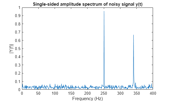
Find frequency components of a signal in additive noise.

Fs = 800; L = 1000; t = (0:L-1)'/Fs; x = sin(2pi250t) + 0.75cos(2pi340t); y = x + .5randn(size(x)); % noisy signal ft = dsp.FFT(FFTLengthSource="Property", ... FFTLength=1024); Y = ft(y);

Plot the single-sided amplitude spectrum

plot(Fs/2linspace(0,1,512), 2abs(Y(1:512)/1024)) title("Single-sided amplitude spectrum of noisy signal y(t)") xlabel("Frequency (Hz)"); ylabel("|Y(f)|")

Figure contains an axes object. The axes object with title Single-sided amplitude spectrum of noisy signal y(t), xlabel Frequency (Hz), ylabel |Y(f)| contains an object of type line.

Compute the FFT of a noisy sinusoidal input signal. The energy of the signal is stored as the magnitude square of the FFT coefficients. Determine the FFT coefficients which occupy 99.99% of the signal energy and reconstruct the time-domain signal by taking the IFFT of these coefficients. Compare the reconstructed signal with the original signal.

Consider a time-domain signal x[n], which is defined over the finite time interval 0≤n≤N-1. The energy of the signal x[n] is given by the following equation:

EN = ∑n=0N-1|x[n]|2

FFT coefficients, X[k], are considered signal values in the frequency domain. The energy of the signal x[n] in the frequency-domain is therefore the sum of the squares of the magnitude of the FFT coefficients:

EN = 1N∑k=0N-1|X[k]|2

According to Parseval's theorem, the total energy of the signal in time or frequency-domain is the same.

EN = ∑n=0N-1|x[n]|2 = 1N∑k=0N-1|X[k]|2

Initialization

Initialize a dsp.SineWave System object to generate a sine wave sampled at 44.1 kHz and has a frequency of 1000 Hz. Construct a dsp.FFT and dsp.IFFT objects to compute the FFT and the IFFT of the input signal.

The FFTLengthSource property of each of these transform objects is set to "Auto". The FFT length is hence considered as the input frame size. The input frame size in this example is 1020, which is not a power of 2, so select the FFTImplementation as "FFTW".

L = 1020; Sineobject = dsp.SineWave(SamplesPerFrame=L,... PhaseOffset=10,... SampleRate=44100,... Frequency=1000); ft = dsp.FFT(FFTImplementation="FFTW"); ift = dsp.IFFT(FFTImplementation="FFTW",... ConjugateSymmetricInput=true); rng(1);

Streaming

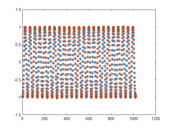
Stream in the noisy input signal. Compute the FFT of each frame and determine the coefficients that constitute 99.99% energy of the signal. Take IFFT of these coefficients to reconstruct the time-domain signal.

numIter = 1000; for Iter = 1:numIter Sinewave1 = Sineobject(); Input = Sinewave1 + 0.01*randn(size(Sinewave1)); FFTCoeff = ft(Input); FFTCoeffMagSq = abs(FFTCoeff).^2;

EnergyFreqDomain = (1/L)*sum(FFTCoeffMagSq);
[FFTCoeffSorted, ind] = sort(((1/L)*FFTCoeffMagSq),...
    1,"descend");

CumFFTCoeffs = cumsum(FFTCoeffSorted);
EnergyPercent = (CumFFTCoeffs/EnergyFreqDomain)*100;
Vec = find(EnergyPercent > 99.99);
FFTCoeffsModified = zeros(L,1);
FFTCoeffsModified(ind(1:Vec(1))) = FFTCoeff(ind(1:Vec(1)));
ReconstrSignal = ift(FFTCoeffsModified);

end

99.99% of the signal energy can be represented by the number of FFT coefficients given by Vec(1):

The signal is reconstructed efficiently using these coefficients. If you compare the last frame of the reconstructed signal with the original time-domain signal, you can see that the difference is very small and the plots match closely.

max(abs(Input-ReconstrSignal))

plot(Input,"*"); hold on; plot(ReconstrSignal,"o"); hold off;

Figure contains an axes object. The axes object contains 2 objects of type line. One or more of the lines displays its values using only markers

Algorithms

This object implements the algorithm, inputs, and outputs described on the FFT block reference page. The object properties correspond to the block parameters.

References

[2] Frigo, M. and S. G. Johnson, “FFTW: An Adaptive Software Architecture for the FFT,”Proceedings of the International Conference on Acoustics, Speech, and Signal Processing, Vol. 3, 1998, pp. 1381-1384.

Extended Capabilities

expand all

Usage notes and limitations:

System Objects in MATLAB Code Generation (MATLAB Coder).
When the following conditions apply, the executable generated from this System object relies on prebuilt dynamic library files (.dll files) included with MATLAB®:
- FFTImplementation is set to"FFTW".
- FFTImplementation is set to"Auto",FFTLengthSource is set to"Property", andFFTLength is not a power of two.
  Use the packNGo function to package the code generated from this System object and all the relevant files in a compressed zip file. Using this zip file, you can relocate, unpack, and rebuild your project in another development environment where MATLAB is not installed. For more details, see How To Run a Generated Executable Outside MATLAB.
When the FFT length is a power of two, you can generate standalone C and C++ code from this System object.

Version History

Introduced in R2012a