dsp.FIRDecimator - Perform polyphase FIR decimation - MATLAB (original) (raw)
Perform polyphase FIR decimation
Description
The dsp.FIRDecimator System object™ performs an efficient polyphase decimation using an integer downsampling factor_M_ along the first dimension.
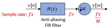
Conceptually, the FIR decimator (as shown in the schematic) consists of an anti-aliasing FIR filter followed by a downsampler.
The FIR filter filters the data in each channel of the input using a direct-form FIR filter. The FIR filter coefficients can be specified through theNumerator property, or can be automatically designed by the object using the designMultirateFIR function. ThedesignMultirateFIR function designs an anti-aliasing FIR filter. The downsampler that follows the FIR filter downsamples each channel of filtered data by taking every _M_-th sample and discarding the M – 1 samples that follow. M is the value of the decimation factor that you specify. The resulting discrete-time signal has a sample rate that is 1/M times the original sample rate.
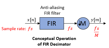
Note that the actual object algorithm implements a direct-form FIR polyphase structure, an efficient equivalent of the combined system depicted in the diagram. For more details, seeAlgorithms.
To resample vector or matrix inputs along the first dimension:
- Create the
dsp.FIRDecimatorobject and set its properties. - Call the object with arguments, as if it were a function.
To learn more about how System objects work, see What Are System Objects?
This object supports C/C++ code generation and SIMD code generation under certain conditions. For more information, see Code Generation.
Creation
Syntax
Description
`firdecim` = dsp.FIRDecimator returns an FIR decimator object with a decimation factor of 2. The object designs the FIR filter coefficients using the designMultirateFIR(1,2) function.
`firdecim` = dsp.FIRDecimator(`M`) returns an FIR decimator with the integer-valued DecimationFactor property set to M. The object designs its filter coefficients based on the decimation factor M that you specify while creating the object, using the designMultirateFIR(1,M) function. The designed filter corresponds to a lowpass with a cutoff at π/M in radial frequency units.
`firdecim` = dsp.FIRDecimator(`M`,`"Auto"`) returns an FIR decimator with the NumeratorSource property set to "Auto". In this mode, every time there is an update in the decimation factor, the object redesigns the filter using designMultirateFIR(1,M).
`firdecim` = dsp.FIRDecimator(`M`,`num`) returns an FIR decimator with theDecimationFactor property set toM and the Numerator property set to num.
`firdecim` = dsp.FIRDecimator(___,`Name=Value`) returns an FIR decimator object with each specified property set to the specified value. For example, to specify a decimation factor of 4, set DecimationFactor to 4.
`firdecim` = dsp.FIRDecimator(`M`,`"legacy"`) returns an FIR decimator where the filter coefficients are designed using fir1(35,0.4). The designed filter has a cutoff frequency of 0.4π radians/sample.
Properties
Unless otherwise indicated, properties are nontunable, which means you cannot change their values after calling the object. Objects lock when you call them, and therelease function unlocks them.
If a property is tunable, you can change its value at any time.
For more information on changing property values, seeSystem Design in MATLAB Using System Objects.
Main Properties
Decimation factor M, specified as a positive integer. The FIR decimator reduces the sampling rate of the input by this factor. The number of input rows must be a multiple of the decimation factor.
Data Types: single | double | int8 | int16 | int32 | int64 | uint8 | uint16 | uint32 | uint64
FIR filter coefficient source, specified as one of the following:
"Property"–– The numerator coefficients are specified through theNumeratorproperty."Input port"–– The numerator coefficients are specified as an input to the object algorithm."Auto"–– The numerator coefficients are designed automatically using thedesignMultirateFIR(1,M)function.
Numerator coefficients of the FIR filter, specified as a row vector in powers of_z–1_. The following equation defines the system function for a filter of length N+1:
The vector b = [b0,b1, …,_bN_] represents the vector of filter coefficients.
To prevent aliasing as a result of downsampling, the filter transfer function should have a normalized cutoff frequency no greater than 1/M. To design an effective anti-aliasing filter, use the designMultirateFIR function. For an example, see Decimate Sum of Sine Waves.
Dependencies
This property is visible only when you setNumeratorSource to"Property".
When NumeratorSource is set to"Auto", the numerator coefficients are automatically redesigned usingdesignMultirateFIR(1,M). To access the filter coefficients in the automatic design mode, type_objName._Numerator in the MATLAB® command prompt.
Data Types: single | double | int8 | int16 | int32 | int64 | uint8 | uint16 | uint32 | uint64
Complex Number Support: Yes
Specify the implementation of the FIR filter as either"Direct form" or "Direct form transposed".
Code Generation Properties
Allow arbitrary frame length for fixed-size input signals in the generated code, specified as true or false. When you specify:
true–– The input frame length does not have to be a multiple of the decimation factor. The output of the object in the generated code is a variable-size array.false–– The input frame length must be a multiple of the decimation factor.
When you specify variable-size signals, the input frame length can be arbitrary and the object ignores this property in the generated code. When you run this object in MATLAB, the object supports arbitrary input frame lengths for fixed-size and variable-size signals and this property does not affect the object behavior.
Data Types: logical
Fixed-Point Properties
Flag to use full-precision rules for fixed-point arithmetic, specified as one of the following:
true–– The object computes all internal arithmetic and output data types using the full-precision rules. These rules provide the most accurate fixed-point numerics. In this mode, other fixed-point properties do not apply. No quantization occurs within the object. Bits are added, as needed, to ensure that no roundoff or overflow occurs.false–– Fixed-point data types are controlled through individual fixed-point property settings.
For more information, see Full Precision for Fixed-Point System Objects and Set System Object Fixed-Point Properties.
Rounding method for fixed-point operations. For more details, see rounding mode.
Dependencies
This property is not visible and has no effect on the numerical results when the following conditions are met:
FullPrecisionOverrideset totrue.FullPrecisionOverrideset tofalse,ProductDataTypeset to"Full precision",AccumulatorDataTypeset to"Full precision", andOutputDataTypeset to"Same as accumulator".
Under these conditions, the object operates in full precision mode.
Overflow action for fixed-point operations, specified as one of the following:
"Wrap"–– The object wraps the result of its fixed-point operations."Saturate"–– The object saturates the result of its fixed-point operations.
For more details on overflow actions, see overflow mode for fixed-point operations.
Dependencies
This property is not visible and has no effect on the numerical results when the following conditions are met:
FullPrecisionOverrideset totrue.FullPrecisionOverrideset tofalse,OutputDataTypeset to"Same as accumulator",ProductDataTypeset to"Full precision", andAccumulatorDataTypeset to"Full precision"
Under these conditions, the object operates in full precision mode.
Data type of the FIR filter coefficients, specified as:
"Same word length as input"–– The word length of the coefficients is the same as that of the input. The fraction length is computed to give the best possible precision."Custom"–– The coefficients data type is specified as a custom numeric type through theCustomCoefficientsDataTypeproperty.
Word and fraction lengths of the coefficients data type, specified as an autosigned numerictype (Fixed-Point Designer) with a word length of 16 and a fraction length of 15.
Dependencies
This property applies when you set theCoefficientsDataType property to"Custom".
Data type of the product output in this object, specified as one of the following:
"Full precision"–– The product output data type has full precision."Same as input"–– The object specifies the product output data type to be the same as that of the input data type."Custom"–– The product output data type is specified as a custom numeric type through theCustomProductDataTypeproperty.
For more information on the product output data type, see Multiplication Data Types.
Dependencies
This property applies when you set FullPrecisionOverride tofalse.
Word and fraction lengths of the product data type, specified as an autosigned numeric type with a word length of 32 and a fraction length of 30.
Dependencies
This property applies only when you setFullPrecisionOverride tofalse andProductDataType to"Custom".
Data type of an accumulation operation in this object, specified as one of the following:
"Full precision"–– The accumulation operation has full precision."Same as product"–– The object specifies the accumulator data type to be the same as that of the product output data type."Same as input"–– The object specifies the accumulator data type to be the same as that of the input data type."Custom"–– The accumulator data type is specified as a custom numeric type through theCustomAccumulatorDataTypeproperty.
Dependencies
This property applies when you set FullPrecisionOverride tofalse.
Word and fraction lengths of the accumulator data type, specified as an autosigned numeric type with a word length of 32 and a fraction length of 30.
Dependencies
This property applies only when you setFullPrecisionOverride tofalse andAccumulatorDataType to"Custom".
Data type of the object output, specified as one of the following:
"Same as accumulator"–– The output data type is the same as that of the accumulator output data type."Same as input"–– The output data type is the same as that of the input data type."Same as product"–– The output data type is the same as that of the product output data type."Custom"–– The output data type is specified as a custom numeric type through theCustomOutputDataTypeproperty.
Dependencies
This property applies when you set FullPrecisionOverride tofalse.
Word and fraction lengths of the output data type, specified as an autosigned numeric type with a word length of 16 and a fraction length of 15.
Dependencies
This property applies only when you setFullPrecisionOverride tofalse andOutputDataType to"Custom".
Usage
Syntax
Description
[y](#d126e288659) = firdecim([x](#d126e288481)) outputs the filtered and downsampled values, y, of the input signal,x.
[y](#d126e288659) = firdecim([x](#d126e288481),[num](#d126e288594)) uses the FIR filter, num, to decimate the input signal. This configuration is valid only when theNumeratorSource property is set to"Input port".
Input Arguments
Data input, specified as a column vector or a matrix of size_P_-by-Q. The columns in the input signal represent Q independent channels.
Under most conditions, the number of inputs rows P can be arbitrary and does not have to be a multiple of theDecimationFactor property. See this table for details.
| Input Signal | When you Run Object in MATLAB | When you Generate Code Using MATLAB Coder™ |
|---|---|---|
| Fixed-size | Object supports arbitrary input frame length | Object supports arbitrary input frame length when you setAllowArbitraryInputLength to true while generating code |
| Variable-size | Object supports arbitrary input frame length | Object supports arbitrary input frame length |
Variable-size signals change in frame length once you lock the object while the fixed-size signals remain constant. When the object does not support arbitrary frame length, the input frame length must be a multiple of theDecimationFactor property.
This object does not support complex unsigned fixed-point inputs.
Data Types: single | double | int8 | int16 | int32 | int64 | uint8 | uint16 | uint32 | uint64 | fi
Complex Number Support: Yes
FIR filter coefficients, specified as a row vector.
Dependencies
This input is accepted only when theNumeratorSource property is set to"Input port".
Data Types: single | double | int8 | int16 | int32 | int64 | uint8 | uint16 | uint32 | uint64 | fi
Complex Number Support: Yes
Output Arguments
FIR decimator output, returned as a column vector or a matrix. When the input is of size _P_-by-Q, and P is not a multiple of the decimation factor M, the output signal has an upper bound size ofceil(P/M)-by-Q. If P is a multiple of the decimation factor, then the output is of size (P/M)-by-Q.
Data Types: single | double | int8 | int16 | int32 | int64 | uint8 | uint16 | uint32 | uint64 | fi
Complex Number Support: Yes
Object Functions
To use an object function, specify the System object as the first input argument. For example, to release system resources of a System object named obj, use this syntax:
| freqz | Frequency response of discrete-time filter System object |
|---|---|
| freqzmr | Compute DTFT approximation of impulse response of multirate or single-rate filter |
| filterAnalyzer | Analyze filters with Filter Analyzer app |
| info | Information about filter System object |
| cost | Estimate cost of implementing filter System object |
| polyphase | Polyphase decomposition of multirate filter |
| impz | Impulse response of discrete-time filter System object |
| coeffs | Returns the filter System object coefficients in a structure |
| outputDelay | Determine output delay of single-rate or multirate filter |
| step | Run System object algorithm |
|---|---|
| release | Release resources and allow changes to System object property values and input characteristics |
| reset | Reset internal states of System object |
Examples
Decimate a sum of sine waves by a factor of 2 and by a factor of 4.
Start with a cosine wave that has an angular frequency of π4 radians/sample.
Design Default Filter
Create a dsp.FIRDecimator object. To prevent aliasing, the object uses an anti-aliasing lowpass filter before downsampling. By default, the anti-aliasing lowpass filter is designed using the designMultirateFIR function. The function designs the filter based on the decimation factor that you specify, and stores the coefficients in the Numerator property. For a decimation factor of 2, the object designs the coefficients using designMultirateFIR(1,2).
firdecim = dsp.FIRDecimator(2)
firdecim = dsp.FIRDecimator with properties:
Main DecimationFactor: 2 NumeratorSource: 'Property' Numerator: [0 -1.0054e-04 0 3.8704e-04 0 -0.0010 0 0.0022 0 -0.0043 0 0.0077 0 -0.0128 0 0.0207 0 -0.0331 0 0.0542 0 -0.1002 0 0.3163 0.5000 0.3163 0 -0.1002 0 0.0542 0 -0.0331 0 0.0207 0 -0.0128 0 0.0077 0 -0.0043 0 0.0022 0 … ] (1×48 double) Structure: 'Direct form'
Show all properties
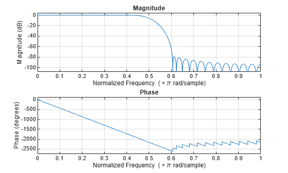
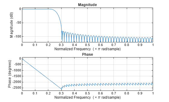
Visualize the filter response. The designed filter meets the ideal filter constraints that are marked in red. The cutoff frequency is approximately half the spectrum.
Decimate by 2
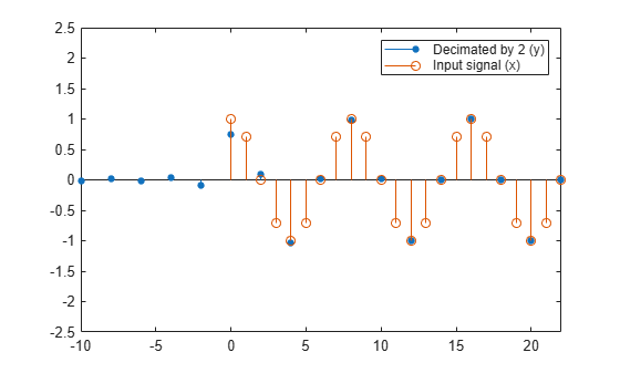
Decimate the cosine signal by a factor of 2.
Plot the original and the decimated signals. In order to plot the two signals on the same plot, you must account for the output delay of the FIR decimator and the scaling introduced by the filter. Use the outputDelay function to compute the delay value introduced by the decimator. Shift the output by this delay value.
Visualize the input and the resampled signals. After a short transition, the output converges to a cosine of frequency π2 as expected, which is twice the frequency of the input signal π4. Due to the decimation factor of 2, the output samples coincide with every other input sample.
[delay,FsOut] = outputDelay(firdecim); nx = (0:length(x)-1); ty = (0:length(y)-1)/FsOut-delay; stem(ty,y,"filled",MarkerSize=4); hold on; stem(nx,x); hold off; xlim([-10,22]) ylim([-2.5 2.5]) legend("Decimated by 2 (y)","Input signal (x)");
Add a High Frequency Component to Input and Decimate
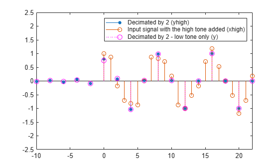
Add another frequency component to the input signal, a sine with an angular frequency of 2π3 radians/sample. Since ω= 2π3 is above the FIR lowpass cutoff, π2, the frequency 2π3 radians/sample is filtered out from the signal.
xhigh = x + 0.2sin(2pi/3*(0:95)'); release(firdecim) yhigh = firdecim(xhigh);
Plot the input signal, decimated signal, and the output of the low frequency component. The decimated signal yhigh has the high frequency component filtered out. yhigh is almost identical to the output of the low frequency component y.
stem(ty,yhigh,"filled",MarkerSize=4); hold on; stem(nx,xhigh); stem(ty,y,":m",MarkerSize=7); hold off; xlim([-10,22]) ylim([-2.5 2.5]) legend("Decimated by 2 (yhigh)",... "Input signal with the high tone added (xhigh)",... "Decimated by 2 - low tone only (y)");
Decimate by 4 in Automatic Filter Design Mode
Now decimate by a factor of 4. In order for the filter design to be updated automatically based on the new decimation factor, set the NumeratorSource property to "Auto". Alternately, you can pass "Auto" as the keyword while creating the object. The object then operates in the automatic filter design mode. Every time there is a change in the decimation factor, the object updates the filter design.
release(firdecim) firdecim.NumeratorSource = "Auto"; firdecim.DecimationFactor = 4
firdecim = dsp.FIRDecimator with properties:
Main DecimationFactor: 4 NumeratorSource: 'Auto' Structure: 'Direct form'
Show all properties
To access the filter coefficients in the automatic mode, type firdecim.Numerator in the MATLAB command prompt.
The designed filter occupies a narrower passband that is approximately a quarter of the spectrum.
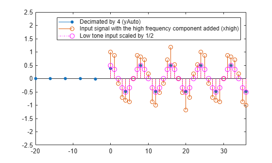
Decimate the cosine signal by a factor of 4. After a short transition, the output converges to a cosine of frequency π as expected, which is four times the lower frequency component of the input signal π4. This time, the amplitude of the output is half the amplitude of the input since the gain of the FIR at ω=π4 is exactly 12. The high frequency component 2π3 diminishes by the lowpass FIR whose cutoff frequency is π4.
Plot the input signal with the high frequency component added, low frequency component scaled by 1/2, and the decimated signal. Recalculate the output delay and the output sample rate since the decimation factor has changed.
[delay,FsOut] = outputDelay(firdecim);
tyAuto = (0:length(yAuto)-1)/FsOut-delay; stem(tyAuto,yAuto,"filled",MarkerSize=4); hold on; stem(nx,xhigh); stem(nx,x/2,"m:",MarkerSize=7); hold off;
xlim([-20,36]) ylim([-2.5 2.5]) legend("Decimated by 4 (yAuto)",... "Input signal with the high frequency component added (xhigh)",... "Low tone input scaled by 1/2");
Reduce the sample rate of an audio signal by a factor of 2 and play the decimated signal using the audioDeviceWriter object.
Note: The audioDeviceWriter System object™ is not supported in MATLAB Online.
Create a dsp.AudioFileReader object. The default audio file read by the object has a sample rate of 22050 Hz.
afr = dsp.AudioFileReader(OutputDataType="single");
Create a dsp.FIRDecimator object and specify the decimation factor to be 2. The object designs the filter using designMultirateFIR(1,2) and stores the coefficients in the Numerator property of the object.
firdecim = dsp.FIRDecimator(2)
firdecim = dsp.FIRDecimator with properties:
Main DecimationFactor: 2 NumeratorSource: 'Property' Numerator: [0 -1.0054e-04 0 3.8704e-04 0 -0.0010 0 0.0022 0 -0.0043 0 0.0077 0 -0.0128 0 0.0207 0 -0.0331 0 0.0542 0 -0.1002 0 0.3163 0.5000 0.3163 0 -0.1002 0 0.0542 0 -0.0331 0 0.0207 0 -0.0128 0 0.0077 0 -0.0043 0 0.0022 0 … ] (1×48 double) Structure: 'Direct form'
Show all properties
Create an audioDeviceWriter object. Specify the sample rate to be 22050/2.
adw = audioDeviceWriter(22050/2)
adw = audioDeviceWriter with properties:
    Device: 'Default'
SampleRate: 11025
Show all properties
Read the audio signal using the file reader object, decimate the signal by a factor of 2, and play the decimated signal.
while ~isDone(afr) frame = afr(); y = firdecim(frame); adw(y); end
release(afr); pause(0.5); release(adw);
More About
A polyphase implementation of an FIR decimator splits the lowpass FIR filter impulse response into M different subfilters, where_M_ is the downsampling or decimation factor. For more details on the polyphase implementation, see Algorithms.
Let h(n) denote the FIR filter impulse response of length N+1 and x(n) the input signal. Decimating the filter output by a factor of M is equivalent to the downsampled convolution:
The key to the efficiency of polyphase filtering is that specific input values are only multiplied by select values of the impulse response in the downsampled convolution. For example, letting M = 2, the input values x(0),x(2),x(4), ... are combined only with the filter coefficients h(0),h(2),h(4),..., and the input values x(1),x(3),x(5), ... are combined only with the filter coefficients h(1),h(3),h(5),.... By splitting the filter coefficients into two polyphase subfilters, no unnecessary computations are performed in the convolution. The outputs of the convolutions with the polyphase subfilters are interleaved and summed to yield the filter output.
The following code demonstrates how to construct the two polyphase subfilters for the default order 35 filter.
M = 2; Num = fir1(35,0.4); FiltLength = length(Num); Num = flipud(Num(:));
if (rem(FiltLength, M) ~= 0) nzeros = M - rem(FiltLength, M); Num = [zeros(nzeros,1); Num]; % Appending zeros end
len = length(Num); nrows = len / M; PolyphaseFilt = flipud(reshape(Num, M, nrows).');
The columns of PolyphaseFilt are subfilters containing the two phases of the filter in Num. For a general downsampling factor of M, there are M phases and therefore M subfilters.
Algorithms
The FIR decimation filter is implemented efficiently using a polyphase structure. For more details on polyphase filters, see Polyphase Subfilters.
To derive the polyphase structure, start with the transfer function of the FIR filter:
N+1 is the length of the FIR filter.
You can rearrange this equation as follows:
M is the number of polyphase components, and its value equals the decimation factor that you specify.
You can write this equation as:
E0(zM),E1(zM), ...,EM-1(zM) are the polyphase components of the FIR filter H(z).
Conceptually, the FIR decimation filter contains a lowpass FIR filter followed by a downsampler.
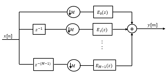
Replace H(z) with its polyphase representation.
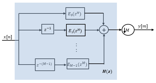
Here is the multirate noble identity for decimation.

Applying the noble identity for decimation moves the downsampling operation to before the filtering operation. This move enables you to filter the signal at a lower rate.
You can replace the delays and the decimation factor at the input with a commutator switch. The switch starts on the first branch 0 and moves in the counterclockwise direction as shown in this diagram. The accumulator at the output receives the processed input samples from each branch of the polyphase structure and accumulates these processed samples until the switch goes to branch 0. When the switch goes to branch 0, the accumulator outputs the accumulated value.
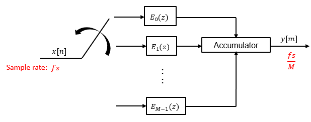
When the first input sample is delivered, the switch feeds this input to the branch 0 and the decimator computes the first output value. As more input samples come in, the switch moves in the counter clockwise direction through branches _M_−1,M_−2, and all the way up to branch 0, delivering one sample at a time to each branch. When the switch comes to branch 0, the decimator outputs the next set of output values. This process continues as data keeps coming in. Every time the switch comes to the branch 0, the decimator outputs y[m]. The decimator effectively outputs one sample for every M samples it receives. Hence the sample rate at the output of the FIR decimation filter is_fs/M.
Extended Capabilities
Usage notes and limitations:
See System Objects in MATLAB Code Generation (MATLAB Coder).
The dsp.FIRDecimator System object supports SIMD code generation using Intel® AVX2 code replacement library under these conditions:
- Filter structure is set to
"Direct form". AllowArbitraryInputLengthproperty is set tofalse.- Input signal is real-valued with real filter coefficients.
- Input signal is complex-valued with real or complex filter coefficients.
- Input signal has a data type of
singleordouble.
The SIMD technology significantly improves the performance of the generated code. For more information, see SIMD Code Generation. To generate SIMD code from this object, see Use Intel AVX2 Code Replacement Library to Generate SIMD Code from MATLAB Algorithms.
For workflow and limitations, see HDL Code Generation for System Objects (HDL Coder).
Note
For a hardware-optimized FIR decimator algorithm that supports HDL code generation, use the dsphdl.FIRDecimator (DSP HDL Toolbox) System object. This object has hardware-friendly valid and reset control signals, and models exact hardware latency behavior. The object supports HDL code generation with HDL Coder™ tools.
Version History
Introduced in R2012a
Starting in R2025a, the Filter Design HDL Coder™ product is discontinued. So, this object no longer supports HDL code generation by using the generatehdl function. The object still supports code generation using HDL Coder tools.
Starting in R2022b, this object supports an input signal with an arbitrary frame length. so the input frame length does not have to be a multiple of the decimation factor.
When you generate code, to support arbitrary frame length for fixed-size signals, you must set the AllowArbitraryInputLength property totrue while generating code.